Scientific Investigations Report 2006-5066
Version 1.0
In cooperation with the U.S. Environmental Protection Agency
1 U.S. Geological Survey, National Wildlife Health Center, Madison, Wis.
This report is available for download as a PDF (14.3 MB)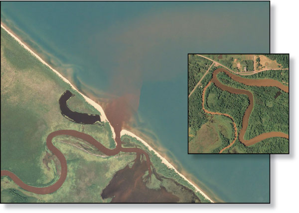
Main photo:
Bad River discharging sediment into Lake Superior near Odanah, Wisconsin
(U.S. Department of Agriculture, 2005)
Inset photo:
Confluence of the White River and Bad River (U.S. Department of Agriculture,
2005)
Abstract
Introduction
Methods
Suspended Sediment Data
Streamflow Data
Load, Yield, and Volumetrically Weighted Concentration Computations
Basin Boundaries and Environmental Characteristics
Statistical Methods
Regional Patterns and Relations to Environmental Factors
Distribution in Water Quality
Median TSS Concentrations
TSS Yields
Volumetrically Weighted TSS Concentrations
Comparisons between Concentrations and Yields
Comparisons of Factors Related to Concentrations and Yields
Comparisons of Reference Concentrations and Yields
Ranking Sites and Prioritizing Rehabilitation Efforts
Summary and Conclusions
Literature Cited
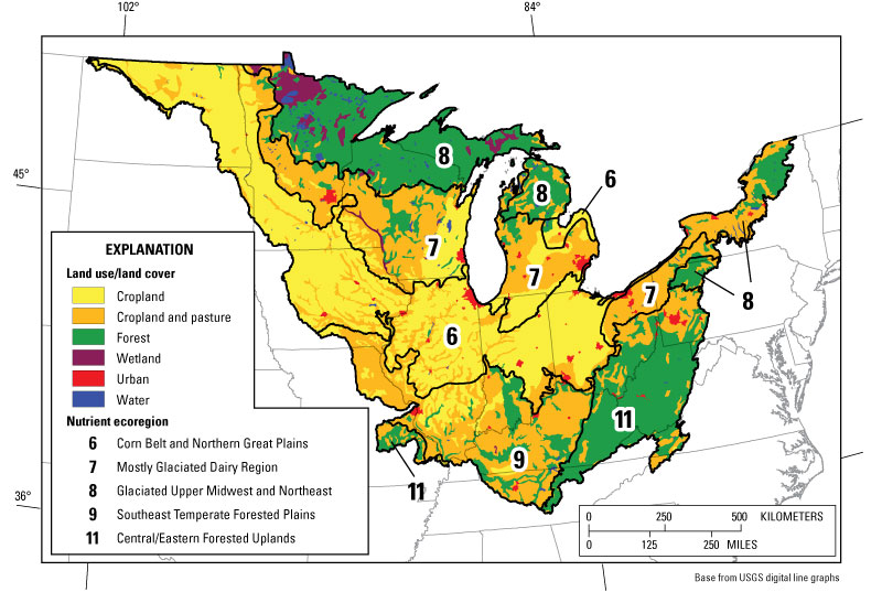
Figure 1. Map showing major land-use/land-cover
categories and national nutrient ecoregions in the study area.
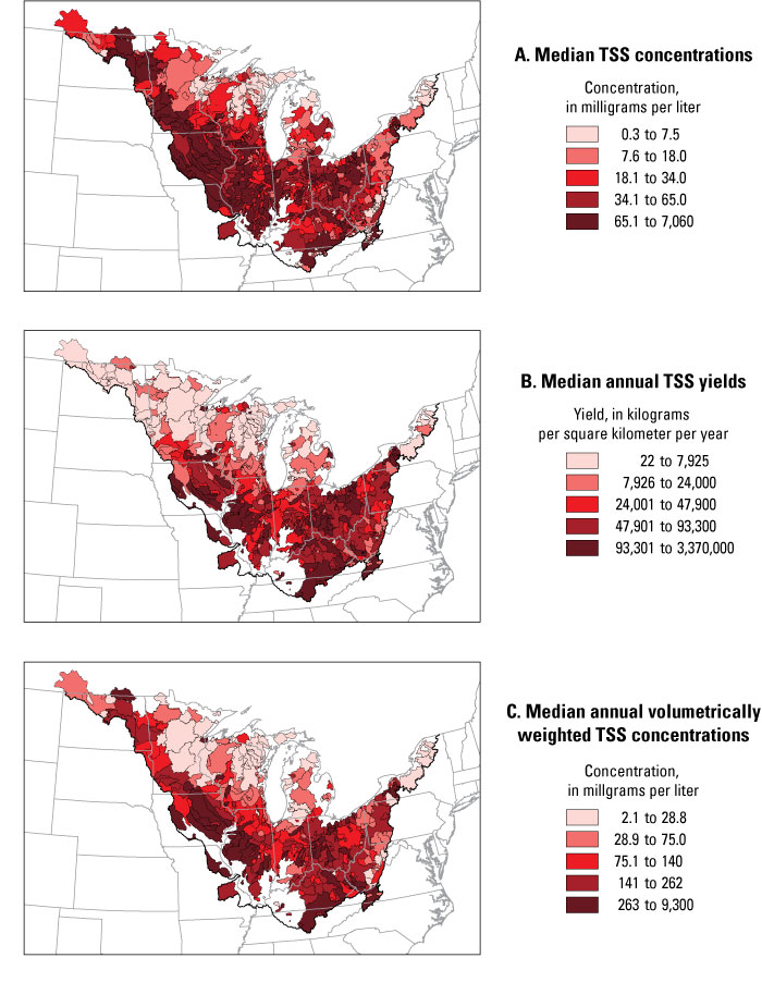
Figure 2. Map showing distributions of
(A) median total suspended sediment/solids (TSS) concentrations, (B) median annual
TSS yields, and (C) median annual volumetrically weighted TSS concentrations
in the study area.
Figure 3. Map showing distributions of
median logarithmically transformed (A) total suspended sediment/solids (TSS)
concentrations, (B) predicted TSS concentrations on the basis of the agricultural
and urban land use in the basin, and (C) land-use-residualized TSS concentrations
in study-area basins.
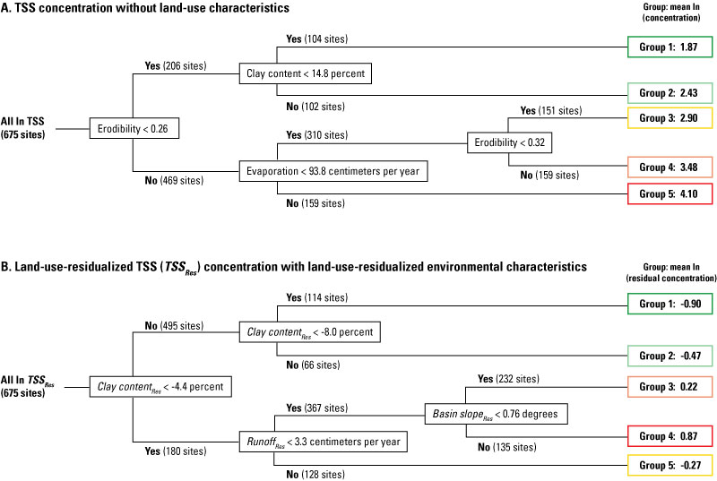
Figure 4. Diagram showing regression-tree analysis results for logarithmically transformed (A) median total suspended sediment/solids (TSS) concentrations and (B) land-use-residualized TSS concentrations.
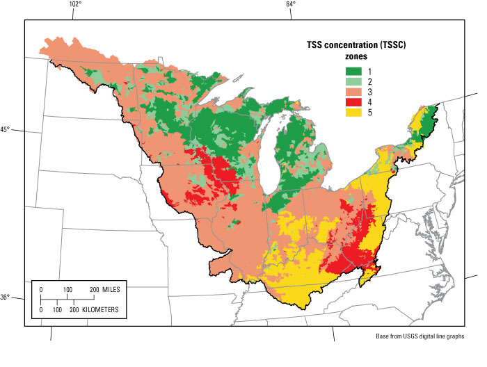
Figure 5. Map showing environmental total suspended sediment/solids (TSS) concentration (TSSC) zones in the study area.
Figure 6. Graph showing response curves for total suspended sediment/solids (TSS) concentrations as a function of the percentage of agriculture in the basin, by environmental TSS concentration (TSSC) zone.
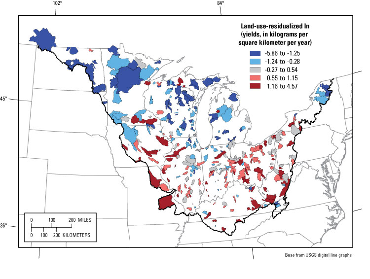
Figure 7. Map showing distributions of land-use-residualized logarithmically transformed annual total suspended sediment/solids (TSS) yields in study-area basins.
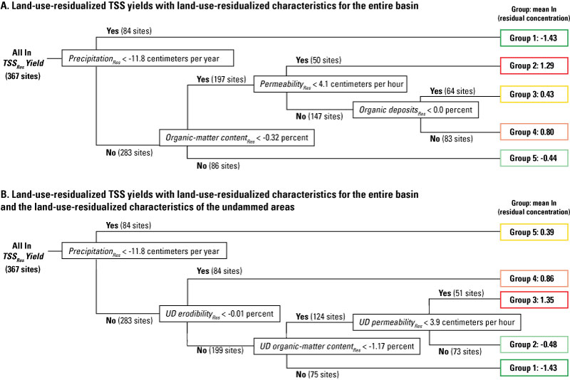
Figure 8. Diagram showing regression-tree results for logarithmically transformed (A) land-use-residualized total suspended sediment/solids (TSS) yields (TSSRes yield) with only land-use-residualized characteristics for the entire basin and (B) TSSRes yield with land-use-residualized characteristics for the entire basin and the land-use-residualized characteristics of the undammed areas.
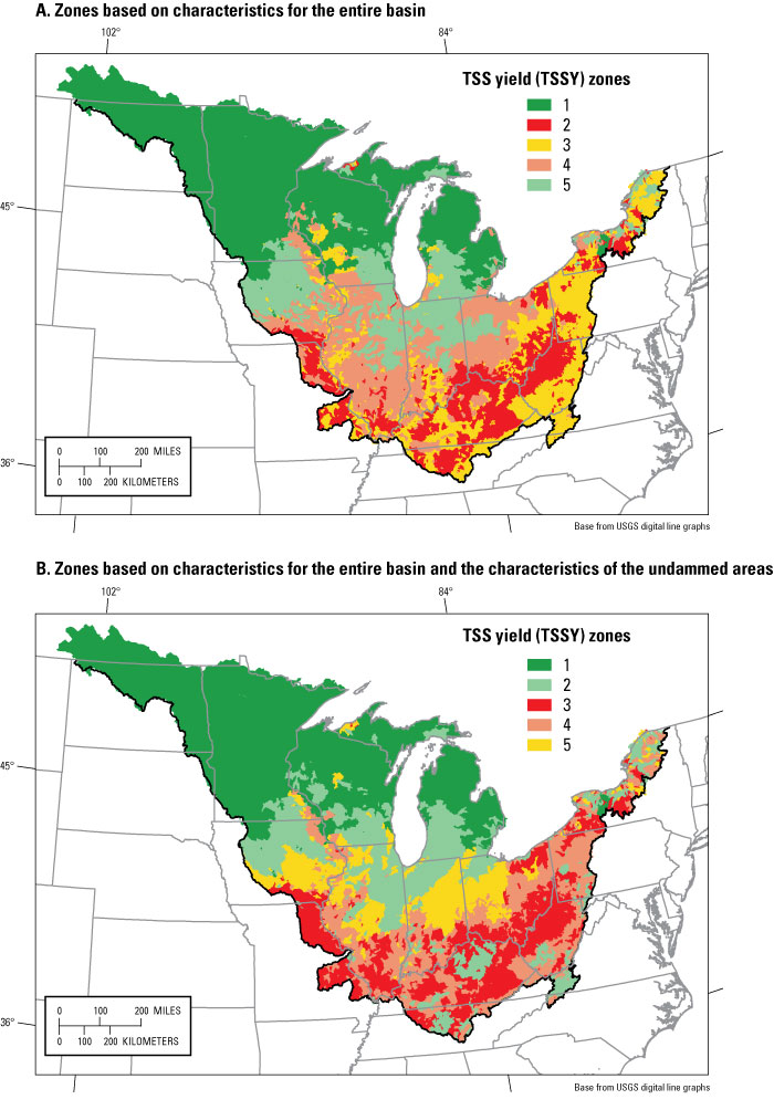
Figure 9. Map showing environmental total suspended sediment/solids yield (TSSY) zones in the study area delineated based on regression-tree results using (A) land-use-residualized characteristics for the entire basin and (B) land-use-residualized characteristics for the entire basin and the land-use-residualized characteristics of the undammed areas.
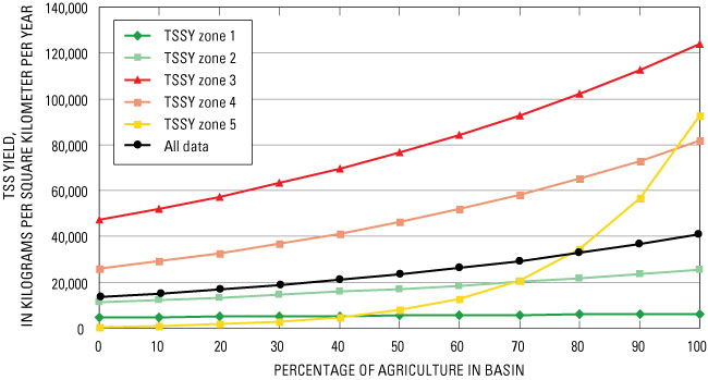
Figure 10. Graph showing response curves for total suspended sediment/solids (TSS) yields as a function of the percentage of agriculture in the basin, by environmental TSS yield (TSSY) zone.
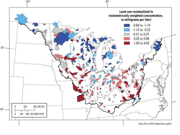
Figure 11. Map showing distributions of land-use-residualized logarithmically transformed volumetrically weighted (VW) total suspended sediment/solids (TSS) concentrations in study-area basins.
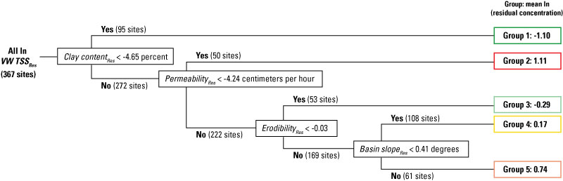
Figure 12. Diagram showing regression-tree results for land-use-residualized volumetrically weighted total suspended sediment/solids (TSSRes) concentrations.
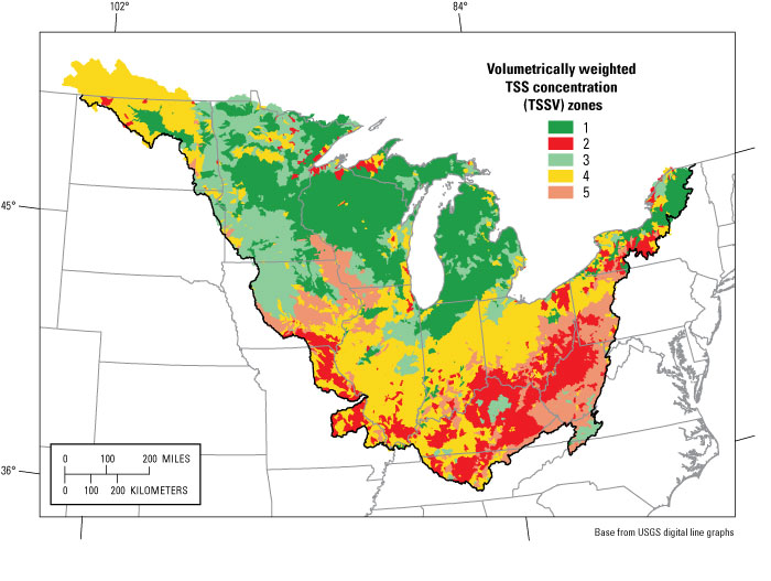
Figure 13. Map showing environmental volumetrically weighted total suspended sediment/solids concentrations (TSSV) zones in the study area.
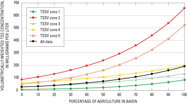
Figure 14. Graph showing response curves for volumetrically weighted (VW) total suspended sediment/solids (TSS) concentrations as a function of the percentage of agriculture in the basin, by VW TSS concentration (TSSV) zone.
Figure 15. Map showing distributions of (A) median total suspended sediment/solids (TSS) concentrations, (B) TSS yields, and (C) volumetrically weighted TSS concentrations exceeding the upper 95th percentile for predicted reference conditions.
Table 2. Pearson correlation coefficients (r) between logarithmically transformed median total suspended sediment/solids (TSS) concentrations, urban area, total agricultural area, and various environmental characteristics, and between land-use-residualized TSS concentrations and land-use-residualized environmental characteristics.
Table 3. Reference median total suspended sediment/solids concentrations (TSSC) and percentiles of all data in various TSSC zones.
Table 4. Pearson correlation coefficients (r) between logarithmically transformed total suspended sediment/solids (TSS) yields, urban area, agricultural area, and various environmental characteristics for the entire basin and characteristics of the undammed area of the basin.
Table 5. Pearson correlation coefficients (r) between selected environmental characteristics of the entire basin for sites with total suspended sediment/solids yields.
Table 6. Reference median annual total suspended sediment/solids yields (TSSY) and percentiles of all data in various TSSY zones.
Table 7. Pearson correlation coefficients (r) between logarithmically transformed volumetrically weighted (VW) total suspended sediment/solids (TSS) concentration, total agricultural area, and various environmental characteristics and between land-use-residualized VW TSS concentration and land-use-residualized environmental characteristics for the entire basin.
Table 8. Reference median annual volumetrically weighted (VW) total suspended sediment/solids concentrations (TSSV) and percentiles of all data in various TSSV zones.
|
Multiply |
By |
To Obtain |
|
Length |
||
| centimeter (cm) | 0.3937 | inch (in.) |
| meter (m) | 3.281 | foot (ft) |
| kilometer (km) | 0.6214 | mile (mi) |
|
Area |
||
| square kilometer (km2) | 247.1 | acre |
| square kilometer (km2) | 0.3861 | square mile (mi2) |
|
Rate |
||
| centimeter per hour (cm/hr) | 0.03281 | foot per hour (ft/hr) |
| centimeter per year (cm/yr) | 0.03281 | foot per year (ft/yr) |
| kilogram per square kilometer (kg/km2) | 5.711 | pound per square mile (lb/mi2) |
|
Mass |
||
| kilogram (kg) | 2.205 | pound avoirdupois (lb) |
Temperature in degrees Celsius (°C) may be converted to degrees Fahrenheit (°F) as follows: °F=(1.8×°C)+32 Concentrations of chemical constituents in water are given either in milligrams per liter (mg/L) or micrograms per liter (μg/L). |
||
Walter (Pete) Redmon, Biologist, U.S. Environmental Protection Agency, Chicago,
Ill.
Gregory E. Schwarz, Economist, U.S. Geological Survey, Reston, Va.
Michael Eberle, Technical Publications Editor, U.S. Geological Survey, Columbus,
Ohio
Jennifer L. Bruce, Geographer, U.S. Geological Survey, Middleton, Wis.
Michelle M. Greenwood, Publications Unit Chief, U.S. Geological Survey, Middleton,
Wis.
In-stream suspended sediment and siltation and downstream sedimentation are common problems in surface waters throughout the United States. The most effective way to improve surface waters impaired by sediments is to reduce the contributions from human activities rather than try to reduce loadings from natural sources. Total suspended sediment/solids (TSS) concentration data were obtained from 964 streams in the Great Lakes, Ohio, Upper Mississippi, and Souris-Red-Rainy River Basins from 1951 to 2002. These data were used to estimate median concentrations, loads, yields, and volumetrically (flow) weighted (VW) concentrations where streamflow data were available. SPAtial Regression-Tree Analysis (SPARTA) was applied to land-use-adjusted (residualized) TSS data and environmental-characteristic data to determine the natural factors that best described the distribution of median and VW TSS concentrations and yields and to delineate zones with similar natural factors affecting TSS, enabling reference or natural concentrations and yields to be estimated.
Soil properties (clay and organic-matter content, erodibility, and permeability), basin slope, and land use (percentage of agriculture) were the factors most strongly related to the distribution of median and VW TSS concentrations. TSS yields were most strongly related to amount of precipitation and the resulting runoff, and secondarily to the factors related to high TSS concentrations. Reference median TSS concentrations ranged from 5 to 26 milligrams per liter (mg/L), reference median annual VW TSS concentrations ranged from 10 to 168 mg/L, and reference TSS yields ranged from about 980 to 90,000 kilograms per square kilometer per year.
Independent streams (streams with no overlapping drainage areas) with TSS data were ranked by how much their water quality exceeded reference concentrations and yields. Most streams exceeding reference conditions were in the central part of the study area, where agricultural activities are the most intensive; however, other sites exceeding reference conditions were identified outside of this area. Whether concentrations or yields should be considered in guiding rehabilitation efforts depends on whether in-stream or downstream effects are more important. Although this study attempted to obtain all available water-quality data for the study area, any actual prioritization of sites for remediation would need to rely on more extensive data collection or numerical models that can accurately simulate the effects of various human activities in a range of environmental settings.
Suspended sediment and siltation are the most common stressors affecting streams throughout the United States (U.S. Environmental Protection Agency, 1998). Suspended sediment reduces the clarity in streams and affects sight-feeding fish; it also interferes with water-treatment processes and recreational uses of streams. Excessive siltation can bury and suffocate fish eggs and bottom-dwelling organisms. In addition to in-stream effects, excessive sediment loading causes sedimentation problems in many downstream lakes and harbors and water-clarity problems in nearshore areas.
The source of much of the sediment and associated nutrients in streams is from upland and streambank erosion. High erosion rates are usually thought to be associated with agricultural activities; however, studies have shown erosion rates to be strongly related to the type of soil and the slope of the terrain in the basin (for example, Monteith and Sonzogni, 1981; Robertson, 1997). Therefore, suspended sediment concentrations in streams are expected to be a function of the soil type, slope of the terrain, and land use in the basin. The load of sediment transported in streams is a function of the concentrations of suspended sediment and the volume of water moving through the stream; therefore, in addition to the factors affecting sediment concentration, precipitation and the resulting runoff also are expected to be important factors.
The most effective way to attain the designated uses of streams impaired by sediments is to reduce the contributions from human activities rather than try to reduce natural loadings. Natural or reference concentrations and loads and their response to human activities (such as agriculture) are expected to vary because of the regional differences in the factors affecting concentrations and loads of suspended sediment. By quantifying reference water quality, basins that are substantially affected by human activities could be more appropriately identified and, therefore, remedial actions could be prioritized.
Several approaches are used to estimate present and reference water quality in streams and describe how water quality responds to various natural and anthropogenic factors. One common approach is to use empirical relations between explanatory factors and specific water-quality characteristics. In this approach, the explanatory factors expected to be related to the distribution of a specific constituent for each monitored stream are defined or quantified and are used to develop empirical equations by use of linear- or nonlinear-regression techniques. This approach has commonly been used to estimate streamflow and chemical concentrations and loads for unmonitored streams (for example, Larson and Gilliom, 2001). Dodds and Oakes (2004) extended this approach to estimate reference water quality by developing multiple linear-regression models relating water quality to various anthropogenic factors such as the percentage of agriculture and percentage of urban area in the basin. The concentration of a constituent occurring in the absence of human activities (for example, 0 percent agriculture and urban areas) then represents the reference concentration. These relations can also be used to place confidence intervals on the estimated reference concentrations. This approach can be used to estimate reference conditions for specific sites or for broader areas having similar environmental characteristics, such as ecoregions (Omernik, 1995).
Various approaches are used to subdivide large areas into regions with similar environmental characteristics that should contain streams with similar reference or natural water quality and that should respond similarly to various factors, such as changes in land use in the basin. For many applications, such as establishing reference conditions, it is preferable to delineate these regions on the basis of physical characteristics that are not affected by human activities. Nevertheless, many approaches, such as ecoregion classifications, often rely on land use to delineate the regions or have difficulties compensating for the effects of land use. Land use not only directly affects water quality but it also is typically correlated with the factors used to define the regions. For example, Robertson and others (2006) have shown land use was the main factor in delineating a set of national nutrient ecoregions in the Midwest (fig. 1; U.S. Environmental Protection Agency, 1998). To remove the effects of land use and delineate zones with similar natural factors affecting water quality, Robertson and others (2006) developed SPAtial Regression-Tree Analysis (SPARTA). In this approach, land-use-adjusted (residualized) water-quality and environmental characteristics are first computed for each site (described in more detail later). Regression-tree analysis (described in more detail later) is then applied to the land-use-residualized data to determine the most statistically important environmental characteristics describing the distribution of a specific water-quality constituent. Geographic information describing the most important environmental characteristics of small basins throughout a study area is then used to subdivide a large area into relatively homogeneous environmental water-quality zones. SPARTA was used to delineate zones of similar reference suspended sediment and total phosphorus concentrations in streams throughout the Great Lakes, Ohio, Upper Mississippi, and Souris-Red-Rainy Basins (Robertson and others, 2006). These zones were shown to describe the differences in reference concentrations better than the national nutrient ecoregions that were delineated primarily by the distributions of different types of land use.
Figure 1. Major land-use/land-cover categories and national nutrient ecoregions (U.S. Environmental Protection Agency, 1998) in the study area.
For each area with relatively similar environmental conditions, several approaches can be used to define its reference water quality and how its water quality responds to changes in land use. Robertson and others (2006) used the regression approach (Dodds and Oakes, 2004) to define reference concentrations for suspended sediment for streams in the various zones in the Great Lakes, Ohio, Upper Mississippi, and Souris-Red-Rainy Basins delineated with SPARTA; however, they did not examine loads, yields, and volumetrically (or flow) weighted (VW) concentrations of suspended sediment. The U.S. Environmental Protection Agency (USEPA) has suggested using the frequency distribution of data available for a specific region to define reference concentrations (U.S. Environmental Protection Agency, 2000). The concentration indicative of reference conditions has been suggested to be the lower 25th percentile of all the data or the upper 75th percentile of a subset of streams thought to be the least affected or impacted by human activity within a defined area.
In 2003, the U.S. Geological Survey (USGS) and the USEPA began a cooperative study in which suspended sediment and suspended solids data collected from 1951 to 2002 in 964 streams throughout the Great Lakes, Ohio, Upper Mississippi, and Souris-Red-Rainy River Basins (Great Lakes region and adjacent areas) of the United States were used to describe the distribution of median concentrations, annual yields (annual load per unit area of the basin), and VW concentrations (total annual load divided total annual flow) of suspended sediment. Spatial regression-tree analyses were used to determine the environmental factors that were most important in describing the distribution of the concentrations and yields of suspended sediment and to delineate zones with similar reference or background median and VW concentrations and yields. A multiple regression approach was used to quantify reference conditions in the various zones and describe how the concentrations and yields in the various zones respond to human activities (changes in the amount of agriculture). The sites were then ranked on the basis of their anthropogenic sources of sediment. The results of this study are summarized in this report.
Water-quality data for this analysis were limited to total suspended sediment and suspended solids concentrations measured in 964 streams in the study area for which sufficient data were available from 1951 to 2002 (described below). For purpose of analysis, total suspended sediment and total suspended solids data were combined into one constituent, TSS. Gray and others (2000) found that total suspended solids were generally less than total suspended sediment by about 25 to 34 percent; however, there was considerable variability in this relation among different areas of the United States. The difference between total suspended sediment and total suspended solids is small compared to spatial differences that exist throughout the study area; therefore, no adjustment factor was applied. These data were assembled from data collected by the USGS and the major sampling agency(s) in each state. USGS data were retrieved from the National Water Information System (NWIS), the National Water-Quality Assessment Program’s Data Warehouse, and the Upper Mississippi Basin Loading database. All of the state-agency data were obtained from USEPA legacy and modernized STORET databases, except data from Illinois (collected by the Illinois Environmental Protection Agency and contained in NWIS), Indiana (collected by the Indiana Department of Environmental Management; C. Bell, written commun., 2002) and Wisconsin (collected by the Wisconsin Department of Natural Resources; J. Ruppel, written commun., 2004).
The number of samples collected at each site was highly variable, and the period of record ranged from 2 years to decades. To compute temporally unbiased median concentrations for each site, the data were subsampled to include only one record per constituent per month per year. The record included in the statistical summaries was the one collected closest to the middle of the month (midmonthly sample). All data reported at less than the detection limit were set to one-half of the detection limit. A selection requirement for a site to be included for a median concentration was that it had at least 15 midmonthly samples. A median concentration was used because medians have been used to establish criteria for streams (U.S. Environmental Protection Agency, 2000), and a median value reduces the effects of outliers and values reported at less than a detection limit. Only independent streams (675 streams) were used in the statistical analyses. Independent streams are those with completely different (nonoverlapping) drainage basins. Additional larger, nonindependent streams were used for graphical purposes.
A selection requirement for a site to be used to compute median annual loads and VW concentrations was that it had at least 25 samples over a period of at least 2 years and at least 5 years of complete daily streamflow records; therefore, a site needed at least 5 years of complete estimated loads to compute a median value. An annual load was computed only if there were no missing daily flows for that year. The requirement of having 5 years of estimated load data to compute median values was used to reduce the potentially large effects of natural climatic variability. Annual VW concentrations were computed by dividing the estimated annual loads by the annual flows. Again, only independent streams were used in the statistical analyses; additional larger streams were used for graphical purposes.
An attempt was made to locate a nearby streamflow gage for each potential load site. A nearby gage is defined as a gage on the same stream or a nearby stream with a drainage-area ratio (water-quality station area divided by gaged area) between about 0.3 and 2.0. Nearby gages with long periods of record were selected over gages with shorter periods of record. In all, 550 sites had sufficient data to compute loads, and 367 of those sites were classified as independent and used for statistical analyses.
Annual loads (calculated by summing daily loads) were estimated by a regression approach by use of the Fluxmaster program (Schwarz and others, 2006) that implements the minimum variance unbiased estimator procedure developed by Cohn and others (1989). In this study, estimated daily loads (L) were computed on the basis of relations between constituent load (in kilograms) and three variables: streamflow (Q, in cubic meters per day), time of the year (T, in radians), and DECTIME (years in decimal format, used to adjust for temporal trends at specific sites). The general form of the model was
| ln(L) = a + b[ln(Q) - c] + d[sin(T)] + e[cos(T)] + f[DECTIME] |
Values for the regression coefficients (a, b, c, d, e, and f ) were computed for each site by the use of multiple-regression analyses between daily loads (daily average streamflows multiplied by instantaneously measured concentrations, in milligrams per liter) and Q, T, and DECTIME. All TSS data from 1951 to 2002 with available corresponding daily streamflows were used in the analysis to estimate the regression coefficients. Daily loads were then estimated for each site from 1971 to 2002. Because a natural logarithmic transformation was used in equation 1, daily loads were adjusted to account for a retransformation bias by use of the minimum variance unbiased estimate procedure (Cohn and others, 1989). Total annual loads were then computed for all years that had no missing daily values (no missing daily flows). Median annual loads, yields, and VW concentrations (total annual load divided by total annual flow) were then computed for each site.
The accuracy of the regression approach to estimate annual loads based on sparse temporal data, as was the case for many of the sites in this study, was evaluated by Robertson (2003). It was found that using this method with more than 23 years of data resulted in median annual loads with standard errors of about 50 percent. Spatial variability in yield and VW concentration data was several orders of magnitude; therefore, the effects of the errors in estimating yields and VW concentrations should be minimal.
Boundaries for most large basins (greater than about 500 km2) were delineated with a geographic information system (GIS) using the USEPA River Reach file (Alexander and others, 1999) and 1-km digital elevation data for North America (Nolan and others, 2002). Boundaries for most small basins were manually digitized from 7.5-minute USGS topographic quadrangle maps or 1:100,000-scale digital coverage of the USGS Hydrologic Unit maps (Seaber and others, 1987) refined with streams included in the National Hydrography Dataset (U.S. Geological Survey, 1999a). The environmental characteristics thought to affect or be related to the TSS in the streams used in this study included land use/land cover (U.S. Geological Survey, 2000), thickness of quaternary deposits (Soller and Packard, 1998), soil characteristics (from the USSOILS digital coverage of the State Soil Geographic (STATSGO) database; Schwarz and Alexander, 1995), types of surficial deposits (Fullerton and others, 2003), annual air temperature and precipitation (National Climatic Data Center, 2002), annual evaporation (Farnsworth and others, 1982), mean land-surface slope (based on 30-m digital elevation model data resampled to 100 m; U.S. Geological Survey, 1999b), and average annual runoff (Gebert and others, 1987). All characteristics were compiled in digital form by use of a GIS and used to compute the average or percentage of each environmental characteristic for each of the 964 basins. A summary of the environmental characteristics for all of the basins used in this study is given in table 1.
Table 1. Summary statistics for total suspended sediment/solids and environmental characteristics examined in the Great Lakes Region and adjacent areas. Summary statistics for land use, surficial deposits, soil properties, and basin characteristics are given for only the independent basins (basins with no overlapping drainage areas).
[TSS, total suspended sediment/solids; VW, volumetrically weighted; N, number of sites; mg/L, milligram per liter; kg/km2, kilogram per square kilometer; %, percent; m, meter; cm/cm, centimeter per centimeter; --, no data or not applicable; cm/hr, centimeter per hour; C, Celsius; cm, centimeter; cm/yr, centimeter per year; km2, square kilometer; mm, millimeter; study area shown in figure 1]
| TSS concentration (mg/L) | ||||||||||||
| All sites (N = 964) | mg/L | 24.0 | 112 | 496 | 0.3 | 7,060 | ||||||
| Independent basins (N = 675) | mg/L | 21.0 | 120 | 566 | 0.3 | 7,060 | ||||||
| TSS annual yields (kg/km2/yr) | ||||||||||||
| All sites (N = 550) | kg/km2 | 35,400 | 85,100 | 226,000 | 22 | 3,373,000 | ||||||
| Independent basins (N = 367) | kg/km2 | 34,700 | 89,500 | 258,000 | 73 | 3,373,000 | ||||||
| TSS annual volumetrically weighted (VW) concentration (mg/L) | ||||||||||||
| All sites (N = 550) | mg/L | 107 | 248 | 654 | 2.1 | 9,300 | ||||||
| Independent basins (N = 367) | mg/L | 98.5 | 267 | 768 | 2.1 | 9,300 | ||||||
| Total forest | % | 26.8 | 38.0 | 32.8 | 0.0 | 100.0 | 22.4 | 33.1 | 29.6 | 0.0 | 100.0 | |
| Total agriculture | % | 57.0 | 51.1 | 34.0 | 0.0 | 98.9 | 66.5 | 55.7 | 32.3 | 0.0 | 98.9 | |
| Total wetland | % | 0.8 | 3.8 | 7.6 | 0.0 | 51.6 | 1.1 | 4.5 | 8.5 | 0.0 | 51.3 | |
| Transitional area | % | 0.0 | 0.2 | 0.5 | 0.0 | 6.2 | 0.0 | 0.1 | 0.4 | 0.0 | 3.1 | |
| Grassland | % | 0.0 | 1.0 | 3.2 | 0.0 | 42.6 | 0.0 | 1.0 | 3.0 | 0.0 | 33.5 | |
| Barren | % | 0.0 | 0.3 | 1.0 | 0.0 | 13.7 | 0.0 | 1.7 | 5.2 | 0.0 | 6.3 | |
| Urban | % | 1.1 | 4.7 | 12.7 | 0.0 | 96.7 | 1.3 | 4.2 | 10.7 | 0.0 | 81.4 | |
| Mean thickness | m | 14.4 | 30.3 | 34.8 | 7.6 | 249.9 | 17.9 | 31.3 | 32.3 | 7.6 | 227.3 | |
| Clay | % | 0.0 | 13.0 | 29.5 | 0.0 | 100.0 | 0.0 | 13.8 | 29.0 | 0.0 | 100.0 | |
| Weathered bedrock | % | 0.0 | 30.2 | 44.3 | 0.0 | 100.0 | 0.0 | 24.5 | 40.7 | 0.0 | 100.0 | |
| Mixed | % | 46.4 | 46.2 | 42.4 | 0.0 | 100.0 | 53.6 | 50.0 | 40.5 | 0.0 | 100.0 | |
| Organic | % | 0.0 | 0.6 | 3.3 | 0.0 | 39.9 | 0.0 | 0.8 | 3.8 | 0.0 | 39.9 | |
| Sand and gravel | % | 0.0 | 10.0 | 20.4 | 0.0 | 100.0 | 0.4 | 10.9 | 19.3 | 0.0 | 100.0 | |
| Available water capacity | cm/cm | 0.14 | 0.14 | 0.03 | 0.07 | 0.23 | 0.15 | 0.15 | 0.03 | 0.07 | 0.23 | |
| Soil erodibility | -- | 0.30 | 0.30 | 0.08 | 0.10 | 0.47 | 0.31 | 0.31 | 0.08 | 0.11 | 0.47 | |
| Clay content1 | % | 24.03 | 23.13 | 8.07 | 3.78 | 53.10 | 25.07 | 23.75 | 7.95 | 3.78 | 44.94 | |
| Organic-matter content2 | % | 1.00 | 2.74 | 3.96 | 0.20 | 24.34 | 1.10 | 2.82 | 3.92 | 0.20 | 21.86 | |
| Permeability | cm/hr | 4.82 | 6.86 | 5.82 | 0.76 | 29.48 | 4.27 | 6.28 | 5.45 | 0.90 | 29.96 | |
| Soil slope | % | 5.93 | 11.78 | 12.48 | 0.64 | 50.90 | 5.37 | 9.30 | 9.83 | 0.64 | 50.90 | |
| Air temperature | degrees C | 9.39 | 9.14 | 2.61 | 2.72 | 14.61 | 9.44 | 9.05 | -15.13 | 2.72 | 14.60 | |
| Precipitation | cm | 96.48 | 97.05 | 17.89 | 39.79 | 167.31 | 96.54 | 96.42 | 17.43 | 43.48 | 167.21 | |
| Evaporation | cm | 83.82 | 84.57 | 9.95 | 92.83 | 106.68 | 83.82 | 85.38 | 9.75 | 68.58 | 106.68 | |
| Precipication minus evaporation | cm | 9.23 | 12.48 | 21.60 | -48.66 | 101.17 | 9.11 | 11.04 | 20.43 | -45.42 | 78.31 | |
| Basin slope | degrees | 1.45 | 3.57 | 4.38 | 0.18 | 20.67 | 1.30 | 2.73 | 3.50 | 0.18 | 19.98 | |
| Runoff | cm/yr | 30.97 | 33.34 | 15.14 | 0.69 | 96.35 | 11.95 | 12.67 | 5.75 | 0.27 | 37.93 | |
| Watershed area | km2 | 241 | 515 | 1,630 | 1.00 | 3,040 | 477 | 1,140 | 2,530 | 1.1 | 30,000 | |
| Undammed area | km2 | -- | -- | -- | -- | -- | 342 | 630 | 1,330 | 0.5 | 21,200 | |
| Undammed fraction | -- | -- | -- | -- | -- | -- | 0.95 | 0.78 | 0.31 | 0.00 | 1.00 | |
In the independent basins with yield data, areas upstream of dams were manually delineated with a GIS based on the locations of dams identified in the “National Inventory of Dams” (U.S. Army Corps of Engineers, 2005) and “Major Dams of the United States” (U.S. Geological Survey, 1999c) and the stream networks included in the National Hydrography Dataset (U.S. Geological Survey, 1999a). Where multiple dams were present within a basin, the most-downstream dam on the main stem or tributary was used to delineate the dammed part of the basin. Dams that were on small headwater streams, and those that were poorly located or poorly attributed were not included in the delineations.
The SAS statistical software package (SAS Institute, Inc., 1989) was used for all statistical analyses except for the regression-tree analyses, which were done by use of the S-PLUS statistical software package (Insightful Corporation, 2001).
Before statistical analyses, all TSS concentrations and yields were logarithmically transformed (natural logarithm). This transformation improved the normality of the data, although not always to the 5-percent significance level (Shapiro-Wilk normality test; Royston, 1982).
A simultaneous partial-residualization approach, related to partial correlation, was used to remove the agricultural and urban effects from the TSS concentrations and yields and each of the environmental characteristics because land use not only directly affects water quality but it also is typically correlated with the environmental characteristics used to define regions of similar water quality. In simple regression, the relationship between a dependent variable Y (for example, TSS concentration) and a predictor X1 (for example, clay content of the soil in the basin) is measured by the sample correlation rYX1. If variable X1 is regressed on the variable X2 (for example, percentage of agriculture in the basin), then the regression equation is X12 = β0 + β1X2. To adjust X1 for the effects of X2, a “residualized X1”, X1Res, is created by computing X1Res = X1 – X12. In a manner similar to simple correlation, the strength of the relation between X1 and Y adjusted for X2 is obtained by the correlation between the residuals for Y on X2 (YRes) and the residuals for X1 on X2 (X1Res). The resulting correlation is the partial correlation of Y and X1 adjusted for X2; that is, the strength of the relation between Y and X1 adjusting for the effects of X2. This approach is easily extended to control for more than one variable; X2 can be replaced by an arbitrary set of variables. In this study, the water-quality constituents and environmental characteristics were adjusted for the percentage of agriculture and urban areas in the basin.
Pearson correlation analyses were done to determine the direction and magnitude of linear relations between each logarithmically transformed water-quality characteristic and the environmental factors. Correlations were done with the original data and with the land-use-residualized data.
In traditional linear-regression analysis, a continuous response variable is assumed to be a linear function of a set of explanatory variables. This assumption is often unrealistic, and departures from linearity can result in underestimating—or completely discounting—the importance of key explanatory variables. Regression-tree analysis (Breiman and others, 1984) avoids these problems by requiring no assumptions about the type of relations between the explanatory variables and response variable. Instead of assuming linear relations, regression-tree analysis sequentially partitions the values of each explanatory variable into two groups, computes mean values of the response variable for each group, and then computes square errors for each partition. At each step, all of response variables are scanned, and the response variable and its breakpoint that minimize the least-square-error criterion are chosen. The least-square-error criterion seeks breakpoints that maximize the variance of interpartition means relative to intrapartition variance. This approach partitions the independent variable space into increasingly homogeneous regions. The end result of this sequential process is a branching diagram.
Regression-tree analyses were done with the original data and the corresponding environmental characteristics data and also with the land-use-residualized water-quality data and the corresponding land-use-residualized environmental characteristic data to determine the most statistically significant environmental characteristics and their breakpoints to describe the distribution of TSS concentrations and yields. In the analysis, the minimum number of observations used to define a subgroup was set to 50 to avoid small outlier groups.
Regression-tree results not only identify the environmental characteristics most strongly related to water quality; of additional importance is that the values used to define the branches can be used to guide the spatial delineation of regions or zones with similar environmental characteristics. Spatially delineating the regions (SPA) from the results of the regression-tree analyses (RTA) led to the process referred to as SPARTA (Robertson and Saad, 2003). To delineate these zones, the study area was first subdivided into approximately 10,000 small drainage basins (mean area of 144 km2) using the USEPA River Reach file (Alexander and others, 1999) and 1-km digital elevation data for North America (Nolan and others, 2002) and the environmental characteristics of each basin were computed with a GIS. Then, each of the 10,000 basins was classified into a specific environmental water-quality zone on the basis of the regression-tree results.
In this study, the residualization process was used to adjust all of the non-land-use variables for the average effects of agriculture and urban areas in the basin. The resulting land-use-residualized concentrations (or yields) of the response variable reflect differences from what would be expected given the land use in the basins. These differences can be associated with differences in the reference concentrations (where the percentages of agriculture and urban areas in the basin are zero) or differences in the response throughout a range in land uses (percentages of agriculture and urban areas) in the study area. Therefore, applying SPARTA to the land-use-residualized data should result in areas of different reference concentrations and (or) areas with different responses to changes in land use. Because factors influencing median TSS concentrations, yields, and VW concentrations may differ, the zones of similar environmental characteristics for each constituent also may differ.
Median midmonthly TSS concentrations ranged from 0.3 to 7,060 mg/L (table 1). The overall median and mean were 24.0 and 112 mg/L, respectively (21.0 and 120 mg/L, for independent basins). Highest concentrations were in the western, southwestern, and south-central parts of the study area (fig. 2A). Lowest concentrations were mostly in northern areas of Wisconsin and Michigan and in the northeastern part of the study area.
Figure 2. Distributions of (A) median total suspended sediment/solids (TSS) concentrations, (B) median annual TSS yields, and (C) median annual volumetrically weighted TSS concentrations in the study area.
Median annual TSS yields ranged from 22 to 3,373,000 kg/km2 (table 1). The overall median and mean were 35,400 and 85,100 kg/km2, respectively (34,700 to 89,500 kg/km2 for independent basins). Highest yields were throughout the southern half of the study area (fig. 2B). Lowest yields were throughout the northern half of the study area. The major difference in the distributions in concentrations and yields was in the northwestern part of the study area, which had high concentrations but low yields.
Median annual VW TSS concentrations ranged from 2.1 to 9,300 mg/L (table 1). The overall median and mean were 107 and 248 mg/L, respectively (98.5 to 267 mg/L for independent basins). The distribution in VW concentrations was similar to that for median concentrations, with the highest concentrations along the western side of the study area (North Dakota, southern Minnesota) and through the central part of the study area (fig. 2C). The highest VW concentrations shifted a little south compared to the median concentrations. Lowest concentrations were in northern areas of Minnesota, Wisconsin, and Michigan and in the northeastern part of the study area.
Patterns in median and VW concentrations closely resembled those of the agricultural areas in the study area (fig. 1), with highest concentrations corresponding to areas with either cropland or cropland and pasture. The major difference was in the southeastern part of the study area, where agriculture is not widespread, yet relatively high concentrations were measured. TSS yields were much less related to agriculture than were concentrations. Low yields were found in the northwestern part of the study area, which is mostly cropland, and high yields were found in the southeast part, which is mostly forested.
Pearson correlation coefficients (r values) between logarithmically transformed median TSS concentrations (fig. 3A) and each environmental factor are listed in table 2 (based on data for 675 independent streams only). Concentrations were significantly correlated with many environmental variables; however, they were most highly correlated with factors describing the basin’s soil properties, evaporation, runoff, and percentage of agriculture. Many of the environmental characteristics (evaporation, precipitation, basin slope, and several surficial-deposit characteristics and soil properties) were strongly correlated with land use, mainly the percentage of agriculture and forest in the basin. For example, evaporation had an r value of 0.66 with the percentage of agriculture (table 2). Therefore, even if the land-use characteristics were not used in further statistical analyses, their effects could be incorporated into the final results by using variables such as evaporation.
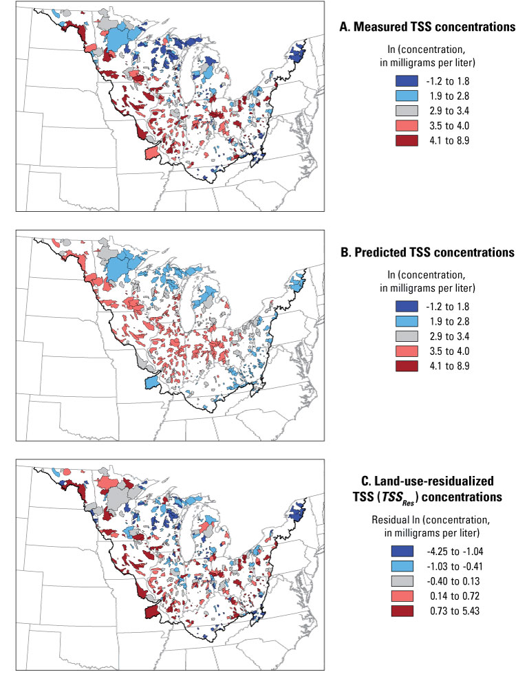
Figure 3. Distributions of median logarithmically transformed (natural logarithm)
(A) total suspended sediment/solids (TSS) concentrations, (B) predicted TSS concentrations
on the basis of the agricultural and urban land use in the basin, and (C) land-use-residualized
TSS concentrations in study-area basins.
Table 2. Pearson correlation coefficients (r) between logarithmically transformed median total suspended sediment/solids (TSS) concentrations, urban area, total agricultural area, and various environmental characteristics, and between land-use-residualized TSS concentrations and land-use-residualized environmental characteristics.
[r values with an absolute value greater than 0.08 are significant at p less than 0.05 with 675 sites; --, not applicable; ln, natural logarithm; r values with an absolute value greater than 0.25 are in bold]
(TSS concentrations) |
agricultural area |
with residual variables |
||
| Total forest | ||||
| Total agriculture | ||||
| Total wetland | ||||
| Transitional area | ||||
| Grassland | ||||
| Barren | ||||
| Urban | ||||
| Mean thickness | ||||
| Clay | ||||
| Weathered bedrock | ||||
| Mixed | ||||
| Organic | ||||
| Sand and gravel | ||||
| Available water capacity | ||||
| Soil erodibility | ||||
| Clay content | ||||
| Organic-matter content | ||||
| Permeability | ||||
| Soil slope | ||||
| Air temperature | ||||
| Precipitation | ||||
| Evaporation | ||||
| Precipitation minus evaporation | ||||
| Basin slope | ||||
| Runoff | ||||
| Watershed area – ln transformed | ||||
To remove the effects of land use from median TSS concentrations and from each environmental characteristic, a simultaneous partial-residualization analysis was done with the percentages of agriculture (Ag%) and urban (Urb%) areas in the basin. Land-use-residualized TSS concentrations (TSSRes) were obtained with
| lnTSSRes = lnTSSMeasured – lnTSSPredicted | ||
| where | lnTSSPredicted = 2.273 + 0.015Ag% + 0.015Urb% (r2 = 0.12) |
The distribution of predicted median TSS concentrations (fig. 3B) closely resembled the land-use patterns in figure 1. After the relations with agriculture and urban land use were removed, high TSSRes were found throughout the entire study area but were still primarily in the western and southern parts (fig. 3C). Residual transformations were also done on all of the environmental characteristics.
Pearson correlation coefficients between TSSRes concentrations and the land-use-residualized environmental characteristics are listed in table 2. TSSRes concentrations were still strongly correlated with many land-use-residualized soil properties and basin slope. Soil erodibility remained the variable most strongly correlated with TSS concentrations. Several characteristics that were strongly correlated to median concentrations were much less correlated to land-use-residualized concentrations; for example, evaporation and runoff.
Regression-tree analyses were done with all environmental characteristics except characteristics describing land use to try to determine which natural environmental characteristics were most statistically significant in describing the distribution of median TSS concentrations (fig. 4A). Soil erodibility was the independent variable chosen for the first subdivision. In that first subdivision, the two groups were sites with erodibility less than (<) 0.26 or greater than or equal to (≥) 0.26. The subgroup with erodibility < 0.26 was further subdivided on the basis of whether the soil clay content was < 14.8 percent (group 1, with 104 sites and the lowest mean ln concentration of 1.87) or ≥ 14.8 percent (group 2, with 102 sites and second lowest mean concentration). The subgroup with erodibility ≥ 0.26 was further subdivided into sites with evaporation < 93.8 cm/yr or ≥ 93.8 cm/yr (group 5, with 159 sites and the highest mean ln concentration of 4.10). The subgroup with evaporation < 93.8 cm/yr was further subdivided into sites with erodibility < 0.32 (group 3, with 151 sites) and ≥ 0.32 (group 4, with 159 sites and second highest mean concentration).
Figure 4. Regression-tree analysis results for logarithmically transformed (A) median total suspended sediment/solids (TSS) concentrations (land-use characteristics were excluded from the analysis) and (B) land-use-residualized TSS concentrations. Final groups are color-coded on the basis of mean concentrations or mean land-use-residualized concentrations from green (lowest) to red (highest).
Although land-use characteristics were not directly included in the regression-tree analysis, they may have indirectly affected the results because of their strong correlations with evaporation. Therefore, to remove the effects of the correlations with land use, regression-tree analysis was applied with the TSSRes data and land-use-residualized environmental characteristic data (fig. 4B). Residualized soil clay content (clayRes) was now the independent variable chosen for the first subdivision. In that first subdivision, the two groups were sites with clayRes< or ≥ -4.4 percent. The subgroup with clayRes < -4.4 percent was further subdivided on the basis of whether clayRes was < -8.0 percent (group 1, with 114 sites and residuals representing the lowest mean TSSRes concentration) or ≥ -8.0 percent (group 2, with 66 sites and residuals representing the second lowest concentration). The subgroup with clayRes ≥ -4.4 percent was further subdivided on the basis of whether the residualized runoff (runoffRes) was < or ≥ 3.3 cm/yr (group 5, with 128 sites). Sites with runoffRes < 3.3 cm/yr were further subdivided into those with residualized basin slope (slopeRes) < 0.76 degrees (group 3, with 232 sites) or slopeRes ≥ 0.76 degrees (group 4, with 135 sites and residuals representing the highest mean concentration). Differences between groups were compared with the Kruskal-Wallis test followed by the Tukey multiple-comparison test. Residual concentrations in group 4 were significantly higher (p < 0.05) than those in group 3, which in turn were significantly higher than those in groups 2 and 5 (which were not significantly different from one another), which in turn were significantly higher than those in group 1. Therefore, although the drainage basins of streams in groups 2 and 5 had different environmental characteristics, their overall effects on TSSRes were similar.
Correlations and regression-tree results indicate that soil properties are the primary natural factors related to the distribution of median TSS concentrations; however, land-use effects may influence the apparent importance of secondary factors such as evaporation. However, simply omitting factors describing land use and reanalyzing the data may or may not give a true indication of secondary factors affecting TSS concentrations because of the correlations of some of these factors with land use. For example, if land-use characteristics are omitted from the analysis, evaporation remains an important factor related to the median TSS distribution. The reason for this is probably not that evaporation directly affects TSS but that a specific evaporation value occurred near the border between mixed cropland and mostly forested areas. After removing the correlations with land use, residualized evaporation was still correlated with residualized TSS, but not as strongly correlated as many other factors. The primary natural factors influencing the distribution of median TSS concentrations were several soil properties (primarily the clay content of the soil) and basin slope.
Results of the regression-tree analysis for TSSRes concentrations were used to classify each of the approximately 10,000 basins in the study area into five specific environmental TSS concentration (TSSC) zones (fig. 5) based on the land-use-residualized characteristics of each basin and the breakpoints defined in figure 4B. Each TSSC zone represents an area having characteristics similar to one of the groups in figure 4B. For example, TSSC zone 1 represents streams in areas with soils having the lowest clay content. By applying SPARTA to the land-use-residualized data, each zone delineates streams that should have similar minimally impacted conditions (similar reference conditions with no agriculture and no urban land) and (or) a similar response to changes in land use.
Figure 5. Environmental total suspended sediment/solids (TSS) concentration (TSSC) zones in the study area. Each zone was delineated on the basis of the results in figure 4B and the land-use-residualized basin characteristics of approximately 10,000 small basins.
To define reference or background concentrations and describe the responses or changes in concentration as a function of land use in each zone, a multiple linear-regression model relating water quality to the percentage of agriculture and urban areas was used (similar to that used by Dodds and Oakes, 2004):
| ln (median TSS concentration) = a Ag% + b Urb% + c | (3) |
where a, b, and c are regression coefficients determined for each zone. With this approach, the concentration of a constituent occurring in the absence of human activities (no agriculture and no urban land) represents the reference concentration. The reference concentration for a zone was estimated as ec, where “e” is the base of the natural system of logarithms. A bias correction is typically applied when logarithmic regression is used; however, it was not used here because the goal was to estimate median reference concentrations rather than mean reference concentrations. All estimated median reference concentrations, standard errors, and 95-percent confidence intervals for the median concentrations are given in table 3.
Median reference TSS concentrations based on the regression approach ranged from about 4 to 6 mg/L in TSSC zones 1 and 2 to 17.2 mg/L in TSSC zones 3 and 4. The upper 95-percent confidence intervals of these estimates ranged from 5.1 mg/L in zone 1 to about 26 mg/L in zones 3 and 4. Lowest reference concentrations (green and light green) were found in central Minnesota, Wisconsin (except for the southeast and southwest parts of these states), Michigan, and the eastern part of the study area (fig. 5). The five zones can be combined into three main categories: TSSC zones 1 and 2 with a reference concentration of about 5 mg/L, zone 5 with a reference concentration of about 9 mg/L, and zones 3 and 4 with a reference concentration of about 17 mg/L. The 95-percent confidence limits for the reference concentrations of zone 5 slightly overlapped with those of the other two main categories.
The USEPA has suggested using the frequency distribution of data available for a specific area to define a reference concentration (U.S. Environmental Protection Agency, 2000). On the basis of the 25th percentile of all of the data in each zone, reference TSS concentrations range from 4 mg/L in TSSC zone 1 to 19 mg/L in zone 3 (table 3). Robertson and others (2006) showed that the effects of the differences in land use within various areas can strongly affect the results of the percentile approach for constituents correlated with land use, such as TSS. Therefore, it is difficult to determine whether the differences between zones 3 and 4 found using the 25th-percentile approach are real or simply an effect of more agriculture in zone 3. Therefore, the values based on the regression approach are considered the more accurate estimates of reference concentrations.
[%, percent; CI, confidence interval; data are concentrations in milligrams per liter]
multiple linear regression |
|||||||||||||
5% CI |
|||||||||||||
The multiple regression equations (eq. 3) used to estimate reference concentrations can also be used to show how changes in land use affect water quality in the different TSSC zones in the study area by adjusting the percentage of agriculture from 0 to 100 percent (fig. 6). The percentage of urban area in a basin was held at zero during the computations. Similar results were obtained when the variable describing the percentage of urban area was completely omitted from the analysis. In general, median TSS concentrations increased as the percentage of agriculture increased in all zones; of substantial interest is the relative difference in how these changes occurred. The major difference is that concentrations in zone 4 increased at a much faster rate than those in the other zones. This indicates that streams in areas dominated by clay soils with relatively low runoff and steep basin slopes have the highest reference TSS concentrations and that increasing agricultural use in this type of environmental setting results in the most rapid increase in concentration. Changes in TSS concentrations as a function of the percentage of agriculture in the other zones were relatively similar. The 90-percent confidence limits for coefficient a (coefficient with Ag%) in equation 3 for zone 4 slightly overlapped with those of all of the other zones.
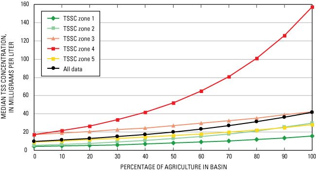
Figure 6. Response curves for total suspended sediment/solids (TSS) concentrations as a function of the percentage of agriculture in the basin, by environmental TSS concentration (TSSC) zone.
Pearson correlation coefficients between ln-transformed TSS yields and each environmental factor are listed in table 4 (based on data for the 367 independent streams only). Annual yields were most highly correlated with soil properties in the basin, air temperature, precipitation, evaporation, and the percentage of wetlands in the basin. Unlike TSS concentrations, yields were only weakly correlated with the percentage of agriculture in the basin; however, many characteristics (such as evaporation, runoff, and several soil properties) were strongly correlated with the percentage of agriculture in the basin.
Table 4. Pearson correlation coefficients (r) between logarithmically transformed total suspended sediment/solids (TSS) yields, urban area, agricultural area, and various environmental characteristics for the entire basin and the undammed area of the basin, and between land-use-residualized TSS yields and land-use-residualized evironmental characteristics for the entire basin and characteristics of the undammed area of the basin.
[r values with an absolute value greater than 0.1 are significant at p less than 0.05 with 367 sites; r values with an absolute value greater than or equal to 0.4 for non-land-use characteristics are in bold; ln, natural logarithm; --, not applicable]
| Basin characteristic | In (TSS yield) | Agricultural area | |||||
| Total forest | |||||||
| Total agriculture | |||||||
| Total wetland | |||||||
| Transitional area | |||||||
| Grassland | |||||||
| Barren | |||||||
| Urban | |||||||
| Mean thickness | |||||||
| Clay | |||||||
| Weathered bedrock | |||||||
| Mixed | |||||||
| Organic | |||||||
| Sand and gravel | |||||||
| Available water capacity | |||||||
| Soil erodibility | |||||||
| Clay content | |||||||
| Organic-matter content | |||||||
| Permeability | |||||||
| Soil slope | |||||||
| Air temperature | |||||||
| Precipitation | |||||||
| Evaporation | |||||||
| Precipitation minus evaporation | |||||||
| Basin slope | |||||||
| Runoff | |||||||
| Watershed area – ln transformed | |||||||
| Undammed ratio | |||||||
To remove the effects of land use from TSS yields and from each environmental characteristic, a simultaneous partial-residualization analysis was done with the percentages of agriculture and urban areas in the basin. The residualization process had a smaller effect on TSS yields than it had on concentrations because of the weaker correlations with the percentage of agriculture. The distribution of land-use-residualized yields for the independent basins (fig. 7) was similar to the untransformed data. TSSRes yields were strongly correlated with most soil properties, air temperature, precipitation, runoff, and basin slope (table 4). The major difference in the correlations with the land-use-residualized variables from the original data was the increase in the r values between TSSRes yields and runoff and with precipitation minus evaporation.
Figure 7. Distributions of land-use-residualized logarithmically transformed (natural logarithm) annual total suspended sediment/solids (TSS) yields in study-area basins.
Reservoirs and other impoundments can greatly reduce the amount of sediment transported down a stream. Therefore, it was hypothesized that the characteristics of the area downstream from impoundments should be more strongly correlated with TSS yields than the characteristics of the entire basin. To test this hypothesis, the environmental characteristics of the area downstream from the impoundments also were determined and examined. Correlation coefficients between logarithmically transformed TSS yields and each environmental factor computed just for the area downstream from the impoundments (undammed area) also are given in table 4. These results were similar to those based on the entire basin for both the original yields and the land-use-residualized yields. This similarity was a result of the environmental characteristics of the undammed areas of each basin being strongly correlated with the environmental characteristics of the entire basin. The smallest Pearson correlation coefficient between the characteristics of the dammed and corresponding characteristic of the undammed areas was 0.93; most coefficients were larger than 0.95.
Although land-use characteristics were not as strongly correlated with yields as they were with concentrations, many correlations were statistically significant; therefore, the land-use-residualized data were used in the regression-tree analysis. Runoff was not included in the analysis because yields are computed as a product of streamflow and concentration and total annual streamflow is approximately equal to runoff, so runoff was not considered an independent explanatory variable. The results of the first analysis with characteristics for the entire basin are given in figure 8A. Residualized precipitation (PPTRes) was the independent variable chosen for the first subdivision. In that first subdivision, the two groups were sites with PPTRes < -11.8 cm/yr (group 1, with 84 sites and residuals representing the lowest yields) or PPTRes ≥ -11.8 cm/yr. The subgroup with PPTRes ≥ -11.8 cm/yr was further subdivided on the basis of whether the residualized percentage of organic-matter content of the soil (OMRes) was < -0.32 percent or ≥ -0.32 percent (group 5, with 86 sites and second lowest residualized yields). The subgroup with OMRes < -0.32 percent was further subdivided on the basis of whether the residualized permeability (permRes) was < -4.1 cm/hr (group 2, with 50 sites and highest residualized yields) or ≥ -4.1 cm/hr. Sites with permRes ≥ -4.1 cm/yr were further subdivided into those with the residualized percentage of organic surficial deposits (ODRes) < 0.00 percent (group 3, with 64 sites) or ODRes ≥ 0.00 percent (group 4, with 83 sites and second highest residualized yields). Residualized yields in group 2 were higher than those in group 4 (not significantly different at p < 0.05 but significantly different at p < 0.1) and were both significantly higher than those in group 3, which in turn were significantly higher than those in group 5, which in turn were significantly higher than those in group 1. Therefore, highest yields were in streams in areas with high precipitation and soils with little organic matter and low permeability.
Regression-tree analysis was then used to examine the relative importance of the environmental characteristics of the entire basin and the undammed areas by including all of the land-use-residualized variables in one analysis (fig. 8B). PPTRes was again the independent variable chosen for the first subdivision. In that division, the two groups were sites with PPTRes < -11.8 cm/yr (group 1, with 84 sites and lowest residualized yields) or PPTRes ≥ -11.8 cm/yr. The subgroup with PPTRes ≥ -11.8 cm/yr was further subdivided on the basis of whether the residualized erodibility of the undammed area (UD erodRes) was < -0.01 (group 2, with 84 sites and second lowest residualized yields) or ≥ -0.01. The subgroup with UD erodRes ≥ -0.01 was further subdivided on the basis of whether the undammed OMRes (UD OMRes) was < -1.17 percent or ≥ -1.17 percent (group 5, with 75 sites). Sites with UD OMRes < -1.17 percent were further subdivided into those with undammed permRes (UD permRes) < 3.9 cm/hr (group 3, with 51 sites and highest residualized yields) and ≥ 3.9 cm/hr (group 4, with 73 sites and second highest residualized yields). Residualized yields in group 3 were higher than those in group 4, which were higher than those in group 5, which were higher than those in group 2, which were higher than those in group 1 (all significant at p < 0.05). Therefore, highest yields were in streams in areas with high precipitation and soils in the areas downstream from the impoundments with high erodibility, low organic-matter content, and low permeability.
Correlations and regression-tree results indicate that precipitation and several soil properties are the major factors related to the distribution of TSS yields. Highest yields were found in streams in areas with high precipitation, especially in areas with highly erodible soils with low permeability and low organic-matter content. Air temperature was the variable most strongly correlated with TSS yields; however, air temperatures were also strongly correlated with precipitation (r = 0.75) and with most of the soil properties that were strongly correlated with yields (r > 0.5). Therefore, it is difficult to interpret the relation between air temperature and TSS yield. The relation between runoff and TSS yields was expected because runoff is part of the yield. TSS yields were most strongly correlated with the types of soils in the undammed areas of the basin, but these soil characteristics are strongly correlated with the characteristics of the entire basin. Therefore, separating these effects is difficult.
Figure 8. Regression-tree results for logarithmically transformed (A) land-use-residualized total suspended sediment/solids (TSS) yields (TSSRes yield) with only land-use-residualized characteristics for the entire basin and (B) TSSRes yield with land-use-residualized characteristics for the entire basin and the land-use-residualized characteristics of the undammed areas. Final groups are color-coded on the basis of mean land-use-residualized yields from green (lowest) to red (highest).
Regression-tree results for land-use-residualized TSS yields based on the characteristics for the entire basin (fig. 8A) and for the entire basin characteristics and the characteristics of the undammed areas (fig. 8B) were used to subdivide the study area into five environmental TSS yield (TSSY) zones (fig. 9). Results of these analyses were used to classify each of the approximately 10,000 basins into specific TSSY zones based on the land-use-residualized characteristics of the entire basin. In the second delineation process, it was assumed that the environmental characteristics upstream from all of the impoundments were similar to those downstream from the impoundments. Most of the characteristics used in the delineation were the variables most strongly correlated with land-use-residualized TSS yields (table 4). Although the two regionalization schemes used different characteristics to delineate the different zones, the final delineation was relatively similar. Both schemes selected residualized precipitation as the most important variable. The reason that the two schemes used different variables in further subdivisions and yet resulted in relatively similar delineation was the strong correlations between the other important explanatory variables (table 5). For example, the second subdivision in one analysis selected on residualized organic-matter content, whereas the other selected on residualized erodibility (r = -0.63 between the nonresidualized data). Organic-matter content, permeability, and erodibility were all strongly correlated with one another.
Table 5. Pearson correlation coefficients (r) between selected environmental characteristics of the entire basin for sites with total suspended sediment/solids yields.
[r values with an absolute value greater than 0.1 are significant at p less than 0.05 with 367 sites; r values with an absolute value greater than 0.5 are in bold]
| Organic deposits | ||||||||
| Soil erodibility | ||||||||
| Clay content | ||||||||
| Organic-matter content | ||||||||
| Permeability | ||||||||
| Air temperature | ||||||||
| Precipitation | ||||||||
| Precipitation minus evaporation |
To define reference yields and describe the responses in yields as a function of the percentage of agriculture in each zone, the multiple linear-regression model (eq. 3) was applied to land-use-residualized TSS yields for each regionalization scheme. All estimated median annual reference yields, standard errors, and the 95-percent confidence intervals are given in table 6. Each regionalization scheme for TSS yields (TSSY) is discussed separately, and the results are then compared.
On the basis of results found using the entire basin characteristics and the regression approach, median reference yields range from 785 kg/km2/yr in TSSY zone 5 to 108,000 kg/km2/yr in zone 4. The upper 95-percent confidence intervals range from 2,610 kg/km2/yr in zone 5 to 341,000 kg/km2/yr in zone 4. The lowest reference yields occur in the central part of the study area (fig. 9A). The five zones can be combined into four main categories: TSSY zone 5 with a reference yield of about 1,000 kg/km2/yr; zone 1 with a reference yield of about 5,000 kg/km2/yr; zones 2 and 3 with a reference yield of about 40,000 kg/km2/yr; and zone 4 with a reference yield of about 100,000 kg/km2/yr. The 95-percent confidence limits for the reference yields of TSSY zones 2, 3, and 4 overlapped with one another.
On the basis of results from the regression approach using both the entire basin characteristics and the characteristics of the undammed areas, median reference yields ranged from 657 kg/km2/yr in TSSY zone 5 to 47,400 kg/km2/yr in zone 3 (table 6). The upper 95-percent confidence intervals ranged from 980 kg/km2/yr in zone 5 to 89,300 kg/km2/yr in zone 3. The standard errors and confidence intervals were smaller than those for the regionalization scheme based on characteristics for the entire basin; therefore, the combination approach is considered the better delineation process for reference yields. Again, the five zones can be combined into four main categories, TSSY zone 5 with a reference yield of about 700 kg/km2/yr, zone 1 with a reference yield of about 5,000 kg/km2/yr, zones 2 and 4 with a reference yield of about 11,000–26,000 kg/km2/yr, and zone 3 with a reference yield of about 45,000 kg/km2/yr. The 95-percent confidence limits for the reference yields of zones 2, 3, and 4 overlapped with one another. Lowest reference yields were again found in the central part of the study area (fig. 9B).
Figure 9. Environmental total suspended sediment/solids yield (TSSY) zones in the study area delineated based on regression-tree results using (A) land-use-residualized characteristics for the entire basin and (B) land-use-residualized characteristics for the entire basin and the land-use-residualized characteristics of the undammed areas. Each zone was delineated on the basis of the results in figure 8 and the residualized basin characteristics of approximately 10,000 small basins.
On the basis of the 25th percentile of all of the data in each zone for both regionalization schemes, reference TSS yields range from about 2,300 to 56,000 kg/km2/yr (table 6). Large differences in land use within the various areas probably affected these results; therefore, the values based on the regression approach are considered the more accurate estimates of reference yields.
Table 6. Reference median annual total suspended sediment/solids yields (TSSY) and percentiles of all data in various TSSY zones.
[%, percent; kg/km2/yr, kilogram per square kilometer per year; CI, confidence interval]
Multiple regression equations (eq. 3) were used to describe how changes in the percentage of agriculture in the basin affect the yields in the different TSSY zones (fig. 10). The response curves are shown only for the regionalization scheme based on results from characteristics from both the entire basin characteristics and the undammed areas (fig. 9B) because the combination approach was considered the better delineation process. TSS yields increased as the percentage of agriculture increased in all zones. The major difference in the responses among zones is that streams in zone 5 had the lowest reference yields, but yields increased at a much faster rate than in the other zones. Zones 3 and 4 had the highest reference yields, but yields increased at moderate rates. Zones 1 and 2 had some of the lowest reference yields, and yields increased at the slowest rates. Streams in zone 5 (fig. 9A), based on results with only the entire basin characteristics used in the regression-tree analysis, also had the lowest reference yields, and they responded most dramatically to increases in agricultural use. Streams in both zone 5s (fig. 9) have relatively high precipitation and high organic-matter content. Streams in both zone 1s have the lowest precipitation and some of the lowest reference yields, and they increased at the slowest rates. The 90-percent confidence limits for coefficient a in equation 3 (agriculture coefficient) for all of the zones except zone 5 overlapped with those of all of the other zones, an indication that many of these differences in response were not statistically significant and that differences in soil properties were more important in affecting yields than the differences in land use.
Figure 10. Response curves for total suspended sediment/solids (TSS) yields as a function of the percentage of agriculture in the basin, by environmental TSS yield (TSSY) zone. The zones were delineated on the basis of regression-tree results using land-use-residualized characteristics of the entire basin and the land-use-residualized characteristics of the undammed areas.
Pearson correlation coefficients between logarithmically transformed VW TSS concentrations and each environmental factor are listed in table 7 (based on data for the 367 independent streams only). VW concentrations were most highly correlated with many of the same factors correlated with median concentrations and yields: soil properties, air temperature, evaporation, and the percentages of agriculture and wetlands in the basin. Unlike median TSS concentrations, VW concentrations were highly correlated with air temperature. Unlike TSS yields, VW concentrations were not highly correlated with runoff or precipitation. VW concentration and many of its correlates were highly correlated with the percentage of agriculture in the basin.
Simultaneous partial residualization was done to remove the land-use effects from the analysis. After the relations with land use were removed, high VW TSSRes concentrations were found throughout the study area; however, most high concentrations were in the southern half (fig. 11). VW TSSRes were most strongly correlated with several soil properties, percentage of sand-and-gravel deposits, and air temperature (table 7). The major difference in the correlations with the land-use-residualized variables was the increase in the r values between VW TSSRes concentrations and soil slope, precipitation, and basin slope.
Figure 11. Distributions of land-use-residualized logarithmically transformed (natural logarithm) volumetrically weighted (VW) total suspended sediment/solids (TSS) concentrations in study-area basins.
Table 7. Pearson correlation coefficients (r) between logarithmically transformed volumetrically weighted (VW) total suspended sediment/solids (TSS) concentration, total agricultural area, and various environmental characteristics and between land-use-residualized VW TSS concentration and land-use-residualized environmental characteristics for the entire basin.
[r values with an absolute value greater than 0.1 are significant at p less than 0.05 with 367 sites; ln, natural logarithm; r values with an absolute value greater than 0.4 are in bold]
(VW TSS concentration) |
area |
with residual variables |
|
| Total forest | |||
| Total agriculture | |||
| Total wetland | |||
| Transitional area | |||
| Grassland | |||
| Barren | |||
| Urban | |||
| Mean thickness | |||
| Clay | |||
| Weathered bedrock | |||
| Mixed | |||
| Organic | |||
| Sand and gravel | |||
| Available water capacity | |||
| Soil erodibility | |||
| Clay content | |||
| Organic-matter content | |||
| Permeability | |||
| Soil slope | |||
| Air temperature | |||
| Precipitation | |||
| Evaporation | |||
| Precipitation minus evaporation | |||
| Basin slope | |||
| Runoff | |||
| Watershed area – ln transformed | |||
| Undammed ratio | |||
Only land-use-residualized VW TSS concentration data were used in the regression-tree analysis (fig. 12). Residualized clay content (clayRes) was the explanatory variable chosen for the first subdivision. In that first subdivision, the two groups were sites with clayRes < -4.65 percent (group 1, with 95 sites and residuals representing the lowest concentrations) or clayRes ≥ -4.65 percent. The subgroup with clayRes ≥ -4.65 percent was further subdivided on the basis of whether permRes was < -4.24 cm/hr (group 2, with 50 sites and residuals representing the highest concentrations) or ≥ -4.24 cm/hr. The subgroup with permRes ≥ -4.24 cm/hr was further subdivided on the basis of whether erodRes was < -0.03 cm/hr (group 3, with 53 sites and second lowest residualized concentrations) or ≥ -0.03. Sites with erodRes ≥ -0.03 were further subdivided into those with the residualized basin slope (slopeRes) < 0.41 degrees (group 4, with 108 sites) or ≥ 0.41 degrees (group 5, with 61 sites and second highest residualized concentrations). The residualized VW concentrations in group 2 were higher than those in group 5 (not significantly different at p < 0.05, but significantly different at p < 0.1) and were both significantly higher than those in group 4, which in turn were significantly higher than those in group 3, which in turn were significantly higher than those in group 1. Therefore, highest VW concentrations were in streams in areas with soils having high clay content and low permeability or in areas with soils having high clay content, low permeability, and high erodibility, and steep basin slopes.
Figure 12. Regression-tree results for land-use-residualized volumetrically weighted total suspended sediment/solids (VW TSSRes) concentrations. Final groups are color-coded on the basis of mean land-use-residualized concentrations from green (lowest) to red (highest).
Correlations and regression-tree results indicate that soil properties and land use are the major factors related to the distribution of VW TSS concentrations. Highest concentrations were in areas with soils having high clay content, low permeability, and high erodibility, and steep basin slopes. Concentrations were especially high if agriculture took place in these areas.
Results of the regression-tree analysis for VW TSSRes concentrations (fig. 12) were used to subdivide the study area into five VW TSS concentration (TSSV) zones (fig. 13). Most of the characteristics used for delineation were the variables most strongly correlated with VW TSSRes concentrations. The regionalization had features found for either median TSS concentrations or TSS yields.
Figure 13. Environmental volumetrically weighted total suspended sediment/solids concentrations (TSSV) zones in the study area. Each zone was delineated on the basis of the results in figure 12 and the land-use-residualized basin characteristics of approximately 10,000 small basins.
Equation 3 was used to define reference median annual VW TSS concentrations and describe the responses in concentrations as a function of land use in each zone. Estimated reference VW concentrations, standard errors, and 95-percent confidence intervals are given in table 8. Reference median VW concentrations ranged from 7.1 mg/L in TSSV zone 1 to 88.1 mg/L in zone 2. The upper 95-percent confidence intervals ranged from 10.2 mg/L in zone 1 to 168 mg/L in zone 2. The lowest reference VW concentrations were found throughout most of Wisconsin and Michigan and the highest VW concentrations were in the southeastern part of the study area. The five zones can be combined into three main categories: TSSV zone 1 with a reference VW concentration of about 7 mg/L, zones 3, 4, and 5 with a reference concentration of about 30–60 mg/L, and zone 2 with a reference concentration of about 90 mg/L. The 95-percent confidence limits for the reference concentrations of zones 3, 4, and 5 overlap with those of zone 2.
Table 8. Reference median annual volumetrically weighted (VW) total suspended sediment/solids concentrations (TSSV) and percentiles of all data in various TSSV zones.
[%, percent; mg/L, milligram per liter; CI, confidence interval; concentrations are shown in milligrams per liter]
of sites |
multiple linear regression |
||||||||||||
5% CI |
95% CI |
error |
|||||||||||
On the basis of the 25th percentile of all of the data in each zone, reference VW TSS concentrations also range from about 8 to 88 mg/L. However, there were large differences in land use within the various areas that may have affected the results; therefore, the values based on the regression approach are considered the more accurate estimates of reference concentrations.
Multiple regression equations (eq. 3) were used to demonstrate how changes in the percentage of agriculture in the basin affect VW TSS concentrations in the different TSSV zones (fig. 14). VW TSS concentrations increase as the percentage of agriculture increases in all of the zones. The major difference in the responses is that the rate of increase in zone 4 was a little less than for the other zones, although none of the rates were significantly different from one another (the 90-percent confidence limits for coefficient a in eq. 3 for all zones overlapped). Reference concentrations of VW TSS concentrations in zones 2 and 5 were among the highest, which resulted in higher VW concentrations at high percentages of agriculture than in the other zones.
Figure 14. Response curves for volumetrically weighted (VW) total suspended sediment/solids (TSS) concentrations as a function of the percentage of agriculture in the basin, by VW TSS concentration (TSSV) zone.
Soil properties and land use were the factors most strongly related to the distribution of median and VW TSS concentrations. Highest concentrations occurred in streams in areas where soils have high clay content, high erodibility, low organic-matter content, low permeability, and steep slopes. Concentrations were especially high if agricultural practices are extensive in these areas. TSS yields were related most strongly to climatic variables (precipitation and runoff) and secondarily related to the factors associated with high TSS concentrations. Highest yields occurred where both precipitation and TSS concentrations were high.
The percentage of agricultural land was strongly correlated with median and VW TSS concentrations and less strongly (but significantly) correlated with TSS yields. The residualization process was important in removing the effects of land use in order that the importance of other factors could be determined. The residualization process was found to be even more important in determining factors influencing constituents that are more strongly related to land use than TSS, such as total phosphorus (Robertson and others, 2006).
It was hypothesized that reservoirs and impoundments may reduce the TSS being transported down a stream. If this was true, then the characteristics downstream from the impoundments may be more influential than the characteristics upstream from the impoundments. TSS yields were found to be most strongly correlated with the types of soils in the undammed areas of the basins. However, these soil characteristics were strongly correlated with similar characteristics computed for the entire basin; therefore, separating these effects was difficult and appeared to have only a small effect on the land-use-regionalization process. Additional information about impoundments, such as their morphometry, age, and retention time, may aid in understanding their effects.
Yields in small streams have been shown to be higher than those in large rivers even if the environmental characteristics of the two basins are similar (Richards, 1989). Because of this finding, delivery coefficients have been added to basin models to describe the loss in sediment and nutrient loads with increasing basin size (Smith and others, 1997). Results of this study indicated that this conclusion is valid; however, the effects of basin size appear to be small. Basin size was only weakly correlated with TSS yields and VW concentrations (r = -0.1) and not correlated with median concentrations.
Lowest reference median and VW TSS concentrations were found for streams in areas having low-clay-content soils, which occur throughout most of Wisconsin and Michigan. Lowest reference yields were found for streams in areas with low precipitation, which occur throughout the northwestern half of the study area, where the lowest reference TSS concentrations also were found. Highest reference median concentrations were found for streams in areas with high-clay-content soils, which occur throughout the western and central parts of the study area. Highest reference VW concentrations and yields were found for streams in the southern and southeastern areas with high precipitation on steep slopes with low-permeability clay soils.
Median TSS concentrations in streams in areas with high-clay-content soils and steep basin slopes were more responsive to increases in the percentage of agriculture than streams in other areas. However, the responses in VW concentrations and yields to increases in the percentage of agriculture were relatively similar among zones except in areas with gentle basin slopes, which were less responsive.
The most effective way to attain the designated uses of surface waters that are currently impaired by sediments is to reduce the contributions from human activities rather than try to reduce natural concentrations and loadings. Prioritization of such efforts could be based on how much the concentration or yield exceeds reference conditions. To determine this, the reference concentrations and yields estimated in this study were subtracted from the measured data at the independent sites, and the sites were then ranked. Although this study attempted to remove all the natural variability in reference conditions by subdividing the study area into zones of similar important environmental characteristics, considerable variability in other factors still exists as demonstrated by the magnitude of the 95-percent confidence limits. Therefore, rather than subtracting the median reference conditions from the measured data, the values at the upper 95-percent confidence limit (tables 3, 6, and 8) were subtracted from the measured data to reduce the potential for identifying sites as impacted when, in fact, their concentrations may reflect natural variability. The sites were then subdivided into five categories: sites not significantly above reference conditions; sites above reference conditions but lower than the 50th percentile of all sites; sites between the 50th and 75th percentiles; sites between the 75th and 90th percentiles; and sites in the upper 10th percentile (fig. 15).
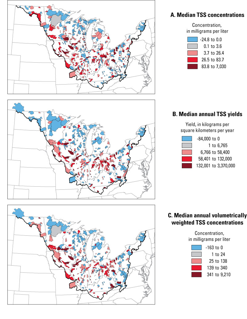
Figure 15. Distributions of (A) median total suspended sediment/solids (TSS) concentrations, (B) TSS yields, and (C) volumetrically weighted TSS concentrations exceeding the upper 95th percentile for predicted reference conditions. Sites are subdivided into five categories: not significantly above reference conditions (light blue), significantly above reference conditions but lower than the 50th percentile of all data (gray), between the 50th and 75th percentiles (pink), between the 75th and 90th percentiles (red), and the upper 10 percent of all sites (maroon).
For median and VW TSS concentrations and TSS yields, most of the sites with concentrations or yields exceeding the upper 75th-percentile values were in the central part of the study area; specifically, in eastern Iowa and western Illinois. For median and VW concentrations, many sites exceeding background concentrations were in southern Wisconsin, the southern half of Minnesota, and North Dakota, whereas for yields, few sites exceeding background conditions were found in central Minnesota and North Dakota. These differences in the distributions in concentrations and yields again demonstrate that land use (agricultural areas) affects concentrations more than it does yields. These maps also identify several basins significantly exceeding reference conditions in areas normally considered relatively pristine, such as in the Upper Peninsula of Michigan. These areas may be affected by other land-use practices, such as logging activities.
All rankings indicate that the streams in the central part of the study area are most affected by anthropogenic factors. However, when using this type of information to guide specific rehabilitative efforts, two questions must be asked: “Which of these data summaries is most important?” and “How do unsampled streams compare to the sampled streams?”
The summary statistics which should be considered depends on how the data will be used. If one is most concerned about the biology in the stream, then the concentrations that typically occur in the stream may be most important, and one may want to consider median concentrations. Median concentrations primarily reflect the concentrations during low flows because low flows occur more frequently than high flows. The amount of TSS being transported down the stream (yield) may be most important if one is concerned about sedimentation in downstream harbors or lakes. Yields would also be very important for nutrients, especially if one was interested in controlling downstream productivity. However, if one is interested in minimizing or controlling the anthropogenic effects on water quality, the most important variable should be the VW concentrations. VW concentrations represent a combination of concentrations during low and high flows. VW concentrations do not reflect the amount of water transported down the stream, which is primarily a function of the amount of precipitation minus evaporation and the type of soils in the basin. Reference and measured VW concentrations were much higher than median concentrations because VW concentrations are more influenced by the higher TSS concentrations that occur during high flows when most of the TSS is transported. Reference median concentrations ranged from 5 to 26 mg/L compared to 10 to 168 mg/L for reference VW concentrations.
Answering the question about unsampled streams compared to the sampled streams is difficult. Although there are distinctive patterns in concentrations and yields, there is also considerable local variability. All three maps in figure 2 show a few sites with relatively low values next to sites with very high values. The relatively low values may be used to test the reference values determined in this study, although even these sites may be impacted. The very high values in some areas suggest that there could also be other sites with very high concentrations and (or) yields that were simply not sampled. Therefore, any actual prioritization of all sites would need to rely on extensive data collection or numerical models that can accurately simulate the effects of various human activities in a range of environmental settings.
In-stream suspended sediment and siltation and downstream sedimentation are common problems in surface waters throughout the United States. The most effective way to improve surface waters impaired by suspended sediments/solids (TSS) is to reduce the contributions from human activities rather than try to reduce loadings from natural sources. Natural or reference TSS concentrations and yields (loads) and their response to human activities vary because of regional differences in the environmental factors affecting their distribution. The main goals of this study, which was performed by the U.S. Geological Survey in cooperation with the U.S. Environmental Protection Agency, were to understand the factors influencing TSS concentrations and yields, and then use this information to delineate zones with similar reference conditions and similar response to changes in land use in the basin. SPAtial Regression-Tree Analysis (SPARTA) was applied to land-use-adjusted (residualized) TSS data and environmental characteristics to determine the natural factors affecting median and volumetrically (flow) weighted (VW) TSS concentrations and yields and to delineate zones with similar natural factors affecting TSS. Reference concentrations and yields were then determined for each zone and used to determine which of the monitored basins were significantly affected by human activities.
Soil properties and land use were the factors most strongly related to the distribution of median and VW TSS concentrations. Highest concentrations were in areas with soils having high clay content, high erodibility, low organic-matter content, and low permeability. Concentrations were especially high if agriculture was extensive in the basins in these areas. TSS yields were most strongly related to precipitation and the resulting runoff and secondarily to the factors related to high TSS concentrations. Yields were highest where precipitation was highest, especially in areas with high TSS concentrations.
Before analysis, all of the data were land-use-adjusted (residualized) to remove the direct and indirect effects of agriculture and urbanization. Regression-tree analysis was then used to determine which natural factors best described the variability in TSS. Breakpoints from the analysis were then used to delineate zones with similar natural factors affecting TSS. These zones were expected to have relatively similar reference conditions and (or) different responses to changes in land use. Because the most important factors influencing TSS concentrations and yields differed, their respective regionalization also differed.
Reference median TSS concentrations ranged from 5 to 26 mg/L, reference median annual VW TSS concentrations ranged from 10 to 168 mg/L, and reference TSS yields ranged from about 980 to 90,000 kg/km2/yr. Lowest reference median and VW TSS concentrations were in areas with low-clay-content soils. Lowest reference yields were in areas with the lowest precipitation, which included the areas with lowest TSS concentrations. Highest reference concentrations were in areas with high-clay-content soils in the western and central parts of the study area, whereas the highest VW concentrations and yields were in areas with high precipitation on steep slopes with low-permeability clay soils. Median TSS concentrations were most responsive to changes in the percentage of agriculture in areas with high-clay-content soils and steep basin slopes. Responses in VW concentrations and yields in most areas were similar except in areas with gentle basin slopes, which were less responsive.
With this information, the independent streams (no overlapping drainage areas) were ranked on the basis of how much their water quality exceeded reference conditions. Most streams significantly exceeding reference conditions were in the central part of the study area, where agricultural activities are the most intensive; however, many sites exceeding reference conditions were also outside of this area. The ranking that should be considered in guiding rehabilitation efforts depends on what is considered most important. If in-stream biology is most important, then median concentrations should be considered. If downstream sedimentation and downstream productivity is most important, then yields should be considered. If one is interested in minimizing or controlling the anthropogenic effects on water quality, then VW concentrations should be considered. Although this study attempted to obtain all available water-quality data for the study area, any actual prioritization for remediation of all sites would need to rely on more extensive data collection or numerical models that can accurately simulate the effects of various human activities in a range of environmental settings.
Alexander, R.B., Brakebill, J.W., Brew, R.E., and Smith, R.A., 1999, ERF1—Enhanced River Reach River 1.2: U.S. Geological Survey Open-File Report 99–457.
Breiman, L., Friedman, J.H., Olshen, R.A., and Stone, C.J., 1984, Classification and regression trees: Belmont, Calif., Wadsworth International Group, 358 p.
Cohn, T.A., DeLong, L.L., Gilroy, E.J., Hirsch, R.M., and Wells, D.K., 1989, Estimating constituent loads: Water Resources Research, v. 25, no. 5, p. 937–942.
Dodds, W.K., and Oakes, R.M., 2004, A technique of establishing reference nutrient concentrations across watersheds affected by humans: Limnology and Oceanography Methods, v. 2, p. 333–341.
Farnsworth, R.K., Thompson, E.S., and Peck, E.L., 1982, Annual free water surface evaporation (shallow lake), 1956–70 in Evaporation atlas for the contiguous 48 United States: National Oceanic and Atmospheric Administration Technical Report NWS 33, Map 3.
Fullerton, D.S., Bush, C.A., and Penne, J.N., 2003, Map of surficial deposits and materials in the eastern and central United States (east of 102 degrees West Longitude): U.S. Geological Survey Geologic Investigations Series I–2789.
Gebert, W.A., Graczyk, D.J., and Krug, W.R., 1987, Average annual runoff in the United States, 1951–80: U.S. Geological Survey Hydrologic Investigation Atlas HA–170, 1 sheet, scale 1:2,000,000.
Gray, J.R., Glysson, G.D., Turcios, L.M., and Schwarz, G.E., 2000, Suspended-sediment concentration and total suspended solids data: U.S. Geological Survey Water-Resources Investigations 00–4191, 14 p.
Insightful Corporation, 2001, S-PLUS 6 for Windows users guide: Seattle, Wash., Insightful Corporation, 688 p.
Larson, S.J., and Gilliom, R.J., 2001, Regression models for estimating herbicide concentrations in U.S. streams from watershed characteristics: Journal of the American Water Resources Association, v. 37, p. 1349–1367.
Monteith, T.J., and Sonzogni, W.A., 1981, Variations in U.S. Great Lakes tributary flows and loading: Great Lakes Basin Commission, Great Lakes Environmental Planning Study Report no. 47, 45 p.
National Climatic Data Center, 2002, Climatography of the U.S.—monthly station normals of temperature, precipitation, and heating and cooling degree days, 1971–2002: Asheville, N.C., National Oceanic and Atmospheric Administration.
Nolan, J.V., Brakebill, J.W., Alexander, R.B., and Schwarz, G.E., 2002. Enhanced river reach file version 2.0: U.S. Geological Survey Open-File Report 02–40.
Omernik, J.M. 1995. Ecoregions—a spatial framework for environmental management, in Davis, W.S., and Simon, T.P., eds., Biological assessment and criteria—tools for water resource planning and decision making: Boca Raton, Fla., Lewis Publishers, p. 49–62.
Richards, R.P., 1989, Evaluation of some approaches to estimating non-point pollutant loads for unmonitored areas: Water Resouces Bulletin, v. 25, no. 4, p. 891–904.
Robertson, D.M., 1997, Regionalized loads of sediment and phosphorus to Lakes Michigan and Superior—high flow and long-term average: Journal of Great Lakes Research, v. 23, p. 416–439.
Robertson, D.M., 2003, Influence of different temporal sampling strategies on estimating total phosphorus and suspended sediment concentration and transport in small streams: Journal of the American Water Resources Association, v. 39, no. 25, p 1281–1310.
Robertson, D.M., and Saad, D.A., 2003, Environmental water-quality zones for streams, a regional classification scheme: Environmental Management, v. 31, p. 581–602.
Robertson, D.M., Saad, D.A., and Heisey, D.M., 2006, A regional classification scheme for estimating reference water quality in streams using land-use-adjusted spatial regression-tree analysis: Environmental Management, v. 37, p. 209-229.
Royston, J.P., 1982, The W test for normality: Applied Statistics, v. 44, p. 176–180.
SAS Institute Inc., 1989, SAS/STAT user’s guide, version 6 (4th ed.): Cary, N.C., SAS Institute Inc.
Schwarz, G.E., and Alexander, R.B., 1995, State Soil Geographic (STATSGO) data base for the conterminous United States: U.S. Geological Survey Open-File Report 95–449.
Schwarz, G.E., Hoos, A.B., Alexander, R.B., and Smith, R.A., 2006, SPARROW-MOD: user documentation for the SPARROW surface water-quality model: U.S. Geological Survey Techniques and Methods, book 6, section B, Surface water, chapter 3 (6–B3).
Seaber, P.R., Kapinos, E.P., and Knapp, G.L., 1987, State hydrologic unit maps: U.S. Geological Survey Water-Supply Paper 2294, 63 p.
Smith, R.A., Schwarz, G.E., and Alexander, R.B., 1997, Regional interpretation of water-quality data: Water Resources Research, v. 33, p. 2781–2798.
Soller, D.R., and Packard, P.H., 1998, Digital representation of a map showing the thickness and character of Quaternary sediments in the glaciated United States east of the Rocky Mountains: U.S. Geological Survey Digital Data Series DDS–38.
U.S. Army Corps of Engineers, 2005, National inventory of dams, water control infrastructure: U.S. Army Corps of Engineers in cooperation with FEMA’s National Dam Safety Program, accessed June 1, 2006, at http://crunch.tec.army.mil/nid/webpages/nid.cfm
U.S. Department of Agriculture, 2005, Wisconsin 2005 National Agriculture Imagery Program photography: U.S. Department of Agriculture, Farm Service Agency, accessed May 30, 2006, at http://www.wisconsinview.org/
U.S. Environmental Protection Agency, 1998, National strategy for the development of regional nutrient criteria: U.S. Environmental Protection Agency, Office of Water, EPA–822–R–98–002, 47 p.
U.S. Environmental Protection Agency, 2000, Nutrient criteria technical guidance manual: rivers and streams: U.S. Environmental Protection Agency, Office of Water, EPA–822–B–00–002, variously paginated.
U.S. Geological Survey, 1999a, National Hydrography Dataset: U.S. Geological Survey Fact Sheet 106–99, accessed June 1, 2006, at http://nhd.usgs.gov/
U.S. Geological Survey, 1999b, National Elevation Dataset: U.S. Geological Survey Fact Sheet 148–99, accessed June 1, 2006, at http://erg.usgs.gov/isb/pubs/factsheets/fs14899.html
U.S. Geological Survey, 1999c, Major dams of the United States: U.S. Geological Survey, accessed June 1, 2006, at http://nationalatlas.gov/mld/dams00x.html
U.S. Geological Survey, 2000, National Land Cover Dataset: U.S. Geological Survey Fact Sheet 108–00, accessed June 1, 2006, at http://erg.usgs.gov/isb/pubs/factsheets/fs10800.html
This report is available online in Portable Document Format (PDF). If you do not have the Adobe Reader, it is available for free download from Adobe Systems Incorporated.
Document Accessibility: Adobe Systems Incorporated has information about PDFs and the visually impaired. This information provides tools to help make PDF files accessible. These tools convert Adobe PDF documents into HTML or ASCII text, which then can be read by a number of common screen-reading programs that synthesize text as audible speech. In addition, an accessible version of Adobe Reader for Windows (English only), which contains support for screen readers, is available. These tools and the accessible reader may be obtained free from Adobe at Adobe Access.
Send questions or comments about this report to the author, Dale M. Robertson, (608) 821-3867.
For more information, visit the Wisconsin Water Science Center.
| AccessibilityFOIAPrivacyPolicies and Notices | |
 |
|