Scientific Investigations Report 2006–5232
U.S. GEOLOGICAL SURVEY
Scientific Investigations Report 2006–5232
Methods of collecting water samples for this study generally followed guidelines established by the USGS and documented in the USGS National Field Manual (U.S. Geological Survey, variously dated), in the USGS Idaho Water Science Center Quality-Assurance Plan for water-quality activities (U.S. Geological Survey, Idaho Water Science Center, written commun., 2005), and in Bartholomay and others (2003). Containerization of purge water necessitated some minor adjustments to the guidelines in Bartholomay and others (2003). It was necessary to split the well discharge into three streams to accommodate sample collection, continuous measurement of the field-water-quality indicators (temperature, pH, specific conductance, and DO), and collection of excess purge water. Excess purge water was collected at the discharge point and routed through canvas hoses to trailer-mounted containers. Containerized purge water was then transported to an approved disposal site near INTEC.
DOE’s Radiological and Environmental Sciences Laboratory (RESL) analyzed water samples for selected radiochemical constituents. A discussion of the procedures used by RESL for the analysis of radionuclides in water samples is provided in reports by Bodner and Percival [eds.] (1982) and U.S. Department of Energy (1995). Analytical methods used by the USGS National Water Quality Laboratory (NWQL) for selected organic and inorganic constituents are described by Goerlitz and Brown (1972), Skougstad and others (1979), Wershaw and others (1987), Fishman and Friedman (1989), Faires (1992), Fishman (1993), and Rose and Schroeder (1995). A list of some analytical methods currently used at the NWQL is available at http://wwwnwql.cr.usgs.gov/Public/ref_list.html. Other analytical methods from the USEPA currently used at the NWQL are available at http://www.epa.gov/epahome/publications.html. Analytical methods from the ASTM that are currently used at the NWQL are available at http://www.astm.org.
Concentrations of radionuclides are reported with an estimated sample standard deviation, s, obtained by propagating sources of analytical uncertainty in measurements. Guidelines for interpreting analytical results for radionuclides are based on an extension of a method by Currie (1984) and are given in a report by Knobel and others (1999). In this report, radionuclide concentrations less than 3s are considered to be below a reporting level.
Water samples were analyzed for the following selected non-radioactive chemical constituents: dissolved trace elements, common ions, nutrients, and purgeable organic compounds. Minimum reporting levels (MRL’s), long-term method detection limits (LT-MDL’s), and laboratory reporting levels (LRL’s), are used by the NWQL to determine when a chemical constituent has been detected with sufficient confidence (Childress and others, 1999).
The MRL is the smallest measured constituent concentration that can be reliably reported using a given analytical method (Timme, 1995). In this report, MRL’s are used only to report concentrations of purgeable organic compounds. The LT-MDL controls false positive error and is determined by calculating the standard deviation of a large sample population (at least 24 measurements) of spiked-sample measurements over an extended period (often 1 year). At the NWQL, the LT-MDL can change on a yearly basis. The chance of falsely reporting a concentration at or greater than the LT-MDL for a sample that did not contain the analyte is predicted to be less than or equal to 1 percent (Childress and others, 1999, p. 19). A falsely reported detection is known as a false positive and is an error of the first type in hypothesis testing. The LRL controls false negative error and is determined so the probability of falsely reporting a non-detection for a sample containing an analyte at a concentration equal to or greater than the LRL is predicted to be less than or equal to 1 percent (Childress and others, 1999, p. 19). Falsely reporting a non-detection is known as a false negative and is an error of the second type in hypothesis testing. The LRL generally is equal to twice the yearly-determined LT-MDL.
Analytes detected at concentrations between the LT-MDL and the LRL that pass identification criteria are estimated. Estimated concentrations are noted with a remark code “E.” These data should be used with the understanding that their uncertainty is greater than data reported without the “E” remark code. For consistency with previous publications, estimated concentrations less than the LRLs are treated as censored data in this report. For censored data used in this report, values are less than the LRL or MRL.
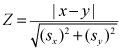
Statistical equivalency of chemical-constituent concentrations in sample pairs was determined following the method outlined by Williams (1996). In this method, statistical equivalence is determined within a specified confidence level. A value for the standard deviate, Z, is calculated, and then the level of significance of the result is evaluated (evaluation of the level of significance assumes that the sample population is distributed normally). For this report, concentrations of individual constituents in sample pairs (constituent pairs) were considered equivalent when the results were within two standard deviations of each other. At this confidence level (95-percent), the level of significance, determined from a standard normal probability curve, was 0.05 for a two-tailed test and corresponded to a Z-value of 1.96.
The equation used to determine Z was adapted from Volk (1969):
 ,
(1)
,
(1)
where
| x | is the concentration of a constituent in the routine sample, |
| y | is the concentration of the same constituent in the sequential replicate sample, |
| sx | is the standard deviation of x, and |
| sy | is the standard deviation of y. |
When the population is not distributed normally or an approximation of the standard deviation is used, a Z-value less than 1.96 must be considered a guide when testing for equivalence. Constituent concentrations in sample pairs were considered statistically equivalent when the calculated Z-value was less than or equal to 1.96. Constituent concentrations also were considered statistically equivalent, although Z-values were not calculated, when the concentration in both samples was reported as less than the LRL or MRL. In this case, the Z-value was reported as zero.
In this report, three types of sample pairs were evaluated for statistical equivalency: (1) a replicate-sample pair collected from well USGS 22 (fig. 1); (2) sample pairs collected after purging 1 and 3 wellbore water volumes at each of 17 wells (figs. 1, 2); and (3) sample pairs collected in an earlier study (Bartholomay, 1993) after purging 1, 2, and 3 wellbore volumes at each of 11 wells (figs. 1, 2). Each sample pair generates multiple constituent pairs.
Using equation 1 is straightforward in determining whether results of radiochemical analyses of a pair of samples were equivalent. RESL reports radionuclide concentrations with an estimated sample standard deviation obtained by propagating sources of analytical uncertainty in measurements. Estimated sample standard deviations can be used directly in equation 1 to calculate a Z-value. Concentrations of radionuclides and measurements of gross radioactivity, estimated sample standard deviations, and calculated Z-values are provided in table 1.
Equation 1 cannot be applied directly to results when no standard deviations or uncertainties are reported by the laboratory. The NWQL does not report standard deviations with analytical results for non-radioactive inorganic constituents. As a result, approximations of standard deviations were used. The USGS Branch of Quality Assurance conducts an Inorganic Blind Sample Program (IBSP) in which reference samples disguised as environmental samples are submitted to the NWQL. Maloney and others (1993) describe the program and present evaluations of the analytical results. Samples sent by the IBSP to the NWQL are prepared from standard reference water samples (SRWS’s). SRWS’s are used by the USGS SRWS project in a round-robin laboratory evaluation program described by Farrar and Long (1997). Until 1988, the SRWS project used means and standard deviations to describe the round-robin data sets. Since 1988, the project used median and F-pseudosigma as a summary of location and variability in data sets. Hoaglin and others (1983) showed that F-pseudosigma yields an unbiased estimate of standard deviation when the data distribution is Gaussian (http://bqs.usgs.gov/bsp/regress.htm).
Mean and median values in the SRWS data sets traditionally were referred to as Most Probable Values (MPV’s). The IBSP uses SRWS data sets to estimate the MPV’s of the IBSP sample mixes. MPV estimates are based on the proportion of the SRWS’s used in making up the sample mixes. Because SRWS data sets are not always Gaussian, the regression equations were derived from a combination of parametric and nonparametric results. Regression equations were derived for each constituent by regressing the appropriate F-psuedosigma or standard deviation against the IBSP MPV using ordinary least squares. Helsel and Hirsch (1992) provided a general model for estimation of ordinary least-squares:
Fσi = βo + β1MPVi + εi i = 1, 2, …, n (2)
where
| Fσi | is the ith observation of the response variable, Fσ, |
| MPVi | is the ith observation of the explanatory variable, MPV, |
| βo | is the intercept, |
| β1 | is the slope, |
| εi | is the random error or residual for the ith observation, and |
| n | is the sample size. |
SRWS project summary data for semi-annual round-robin sample studies during 2004-05 were used by the IBSP to derive regression equations for each constituent. Concentration ranges of the SRWS project summary data sets used, the derived Fσ equations, and the correlations are available at http://bqs.usgs.gov/bsp/regress.htm. F-pseudosigma values were calculated for each analytical result using the regression equations provided by the IBSP. F-pseudosigma values, which correspond to the appropriate time period and concentration range, were then used as an estimate of standard deviations in equation 1 to calculate Z-values. Concentrations of non-radioactive inorganic constituents, F-pseudosigma estimated sample standard deviations, and calculated Z-values are provided in table 2.
The NWQL also does not report standard deviations with analytical results for organic constituents. As a result, approximations of standard deviations were used when appropriate. The Organic Blind Sample Program (OBSP) uses a F-pseudosigma method similar to the method described for non-radioactive inorganic constituents to estimate the sample standard deviations for total organic carbon (TOC) measurements in water samples. The F-pseudosigma equation is available at http://bqs.usgs.gov/OBSP/WY05Plots/TSbodyLC114TOTAL_ORGANIC_CARBON.html. Concentrations of TOC, F-pseudosigma estimated sample standard deviations, and calculated Z-values are provided in table 3. For purgeable organic compounds (POC’s), analytical results were less than the respective MRL’s for 61 sample pairs in each of 3 water samples. As a result, all 183 Z-values for POC’s were set to zero (table 3).

![]() U.S.
Department of the Interior | U.S. Geological
Survey
U.S.
Department of the Interior | U.S. Geological
Survey
Persistent URL: https://pubs.water.usgs.gov/sir20065232
Page Contact Information: Publications Team
Page Last Modified: Thursday, 01-Dec-2016 19:20:14 EST
