Scientific Investigations Report 2007–5008
U.S. GEOLOGICAL SURVEY
Scientific Investigations Report 2007–5008
The first comparison between measured and modeled lake water-surface elevation showed that the inflows initially included in the model did not account for all water entering the reservoir. Additional flows were needed to balance the water budget, especially in the winter during storms. These missing flows could be composed of small ungaged tributaries, overland flow during storms, or ground water seepage. They made up 10.8 percent of the total inflows in 2002, 9.4 percent in 2003, and 20.0 percent for the 2005–06 storms. To account for these ungaged flows, a distributed tributary was added to each branch of the model. The distributed tributary inflows varied through the simulation period, and typically were greatest during storms. In CE‑QUAL-W2, a distributed tributary inflow is apportioned to segments along an entire model branch according to segment surface area. The final modeled water-surface elevations, including the distributed tributary inflows, show good agreement with the measured water-surface elevations for 2002, 2003, and the 2005–06 storms (fig. 4).
The missing inflow was judged to be largely surface water on the basis of TDS and hydrologic information, so the water temperature and water quality of the distributed tributary inflows were estimated as 90 percent surface water and 10 percent ground water. Water temperature and water quality for the surface water component of the distributed tributaries were estimated to be the same as the water temperature and water quality of the major tributary for each branch. Ground water temperature was estimated from annual average air temperature at the lake. Ground water TDS concentrations were estimated by examining data from nearby ground water wells and the results of several preliminary model runs. Ground water suspended sediment concentrations were set to zero.
Reservoir water temperature patterns are controlled by factors such as the temperature of inflows, the amount of outflow, circulation in the lake, heat exchange at the air-water and sediment-water interfaces, solar radiation, light extinction, and mixing by wind. Detroit Lake typically is isothermal and cold at the beginning of the year (fig. 5). In spring, the surface begins to warm, and by summer a thermocline develops, separating warmer, less dense surface water (epilimnion) from cooler, denser, bottom waters (hypolimnion). The thermocline progressively deepens through the summer; this is an important influence on lake circulation through the summer season. In autumn, the water surface cools, lessening the density differences and allowing vertical mixing (“turnover”) to occur. The lake usually is in an isothermal state by the end of the calendar year.
In Detroit Lake, this seasonal pattern in water temperature repeats on an annual basis and was consistent in the modeled time periods (figs. 6, 7, and 8). Despite differing locations and water depths, temperature patterns were similar for all profile sites in the lake. The consistency of the vertical temperature profiles year-to-year and site-to-site within the lake demonstrates the importance of density patterns in creating a vertical structure within the lake. Temperature is the most important factor influencing water density in Detroit Lake, and, therefore, is among the most important factors in determining its circulation patterns.
Wind also is important in creating a well-mixed layer near the lake surface. The stronger the wind, the deeper is the mixed layer. Several of the profiles in figures 6 and 7 show this effect. The profiles on June 19, 2003, for example, show a well-mixed layer 5 or more meters deep, more so near the dam, where the winds typically are stronger. Such spatial differences in wind speed were not provided by the model’s inputs, so the model was unable to capture such subtleties. Overall, however, the model captured the spatial and temporal patterns in the lake’s water temperature and its vertical structure.
Surface waters showed the greatest seasonal variation in temperature and the warmest summer temperatures, while the deepest waters of Detroit Lake remained cold through the summer (fig. 9). As water depth increased, the timing of the seasonal maximum water temperature shifted to later in the year, from early August near the surface to early October at 40 m. Measured temperatures at 9–40 m depth show larger daily variations than those at the surface or near the bottom. This is likely due to those thermistors being stationed closer to the thermocline, the region where the temperature changes rapidly with depth, combined with the phenomenon of the lake’s internal waves caused by wind or short-term variations in water withdrawals, which causes the thermocline to move up and down. Temperatures near the surface have less daily variation owing to the depth of the mixed layer, but have a more chaotic signal that is tied to patterns in the wind, creating some of the short-duration spikes in these data.
The reservoir, with a relatively low-elevation outlet, released cold water through the summer (fig. 10). The heat that was stored in the upper part of the water column during summer was discharged later in the year when the reservoir was drawn down for flood control purposes. Consequently, outflow water temperatures were coolest in winter and spring, stayed cool through summer, and were warmest in autumn. The difference in temperature between the modeled reservoir outflow and the measured temperature on the North Santiam River 6 km downstream (at Niagara) was due in part to air-water heat exchange between the two locations—warming in summer and cooling in autumn. In addition, several small tributaries that enter the river between the reservoir outflow and the measuring location on the North Santiam River at Niagara might contribute to the temperature difference in figure 10.
Goodness-of-fit statistics were calculated between measured data and model output at the same location and time. For water temperature profiles in the lake, comparing modeled and measured water temperatures for the three time periods (2002, 2003, 2005–06) produced ME between -0.02 and -0.48 ºC, MAE between 0.48 and 0.58 ºC, and RMSE between 0.51 and 0.76 ºC (table 3). For the thermistor string near the dam in 2003, comparing modeled and measured water temperatures for all 23 depths produced a ME of 0.24 ºC, a MAE of 0.72 ºC, and a RMSE of 0.99 ºC. Sources of error in simulating water temperature include estimating inflow water temperatures for Kinney and Box Canyon Creeks as well as the ungaged (distributed) tributaries for all simulations, and estimating inflow water temperatures for French Creek for the 2005–06 storm simulations. In addition, measured data showed that light extinction coefficients were elevated in summer coincident with algal blooms. The model, however, did not include algae, and therefore those higher summer light extinctions due to algal activity were not simulated. Despite these sources of error, the goodness-of-fit statistics indicate very good performance by the model in capturing temperature patterns in the lake. Previous CE-QUAl-W2 models have demonstrated the capability of simulating reservoir temperatures to within 1.0 ºC (MAE) (Cole and Wells, 2002). Error greater than that amount is indicative of problems either with the model or the data; MAE of less than 1.0 ºC has become a benchmark for a well-calibrated CE-QUAL-W2 model.
The concentration of total dissolved solids (TDS) represents the sum of all dissolved constituents in water. TDS was included in the Detroit Lake model primarily to more accurately model suspended sediment, because TDS contributes to density gradients in a reservoir. TDS also provides information on lake water quality. CE-QUAL‑W2 considers TDS to be conservative (nonreactive), meaning that its concentration is affected only by inputs, outputs, and hydrodynamic processes, not by chemical or biological processes. Some of the constituents that make up TDS, however, may not be completely conservative. For instance, nutrients may be taken up or excreted by algae, dissolved constituents may precipitate as solids, or solids may dissolve from suspended or bottom sediments. In any case, available data were insufficient to model each dissolved constituent individually in this system.
TDS concentrations in Detroit Lake were fairly homogeneous in winter (fig. 11). Inflow waters in spring had lower dissolved solids concentrations compared to the lake water, and decreased the TDS concentration throughout the lake. Through summer and autumn, the TDS concentrations in the inflows increased. At that time of year, temperature stratification was present in the reservoir, and the higher concentration inflow waters were not mixed into the colder, denser, hypolimnetic water. Later in the year, when the lake turned over, the higher TDS in the epilimnion mixed into the entire lake.
This seasonal cycle in TDS was similar in all modeled time periods (shown as specific conductance in figs. 12, 13, and 14). There were some differences between sampling sites in the lake. For instance, the most upstream site, Mongold, showed the greatest effect from the tributary inflows. At that location, the plume of inflow water generally was at depths of 15–40 m. These influent plumes that enter the lake at specific depths according to their density are important in determining circulation patterns in the regions of these inflows.
Water released from the reservoir outflow reflects the TDS seasonal cycle in the lake, with lowest values in spring and highest values in late autumn and early winter (reported as specific conductance in fig. 15). The overall trends of measured and modeled specific conductance downstream of the dam compare well, despite the fact that measured specific conductance on the North Santiam River at Niagara is 6 km downstream of the modeled reservoir outflow. The measured data were less smooth compared to the modeled outflow. Part of this difference is due to the entrance of several small tributaries between Detroit Dam and Niagara, and part of the difference is due to dam operation. For instance, at Niagara in spring, two short periods occur where the measured specific conductance decreased to about 25 µS/cm. These correspond to periods when no water was released from Detroit Dam, and the small tributaries between Detroit Dam and Niagara appeared to have lower specific conductance values than the reservoir outflow at that time of year. Note that the comparison of specific conductance data downstream of Detroit Dam is better than the same comparison for temperature (fig. 10). This primarily is due to the largely conservative nature of specific conductance; unlike water temperature, it is not affected by exchange processes across the air-water interface.
Calculation of goodness-of-fit statistics for measured specific conductance and specific conductance converted from modeled TDS for the three modeled time periods (2002, 2003, 2005–06) produced MEs between -0.15 and 1.49 µS/cm, MAEs between 1.31 and 2.11 µS/cm, and RMSEs between 2.42 and 3.13 µS/cm (table 3). Sources of error include the estimation of TDS in ungaged inflows and any nonconservative reactions that affect dissolved solids. Overall, though, errors in simulating specific conductance are approximately 5 to 10 percent of measured values in the lake (range of about 27 to 47 µS/cm).
Sediment suspended in the water column is a natural component of lakes and rivers. Excessive concentrations of suspended sediment, however, can impair certain uses. For example, high sediment loads can bury spawning gravels and reduce light penetration into the water column, making it more difficult for fish to find prey. Sediment in water used for drinking water supply can cause taste and odor problems and impair the efficiency and operation of treatment systems. High concentrations of suspended sediment that settle and deposit in a reservoir can reduce the volume available for water storage. Suspended sediment also can contribute surfaces for ion exchange and adsorption between dissolved and particulate phases of various constituents (Horne and Goldman, 1994), and thus act as a storage and transport medium for nutrients, organic contaminants, and trace metals. Suspended sediment concentrations are controlled by factors such as hydrodynamics, sources, density, and settling rates.
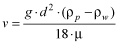
In the model calibration process, the settling rates for the two simulated sediment-size groups were adjusted until the model results and the measured data compared well. In the final Detroit Lake model, suspended sand and silt, particles larger than 2 µm, was given a settling rate of 21.0 m/d, and suspended clay, particles smaller than 2 µm, was given a settling rate of 0.6 m/d. For comparison, Stokes’ Law may be used to estimate the settling velocities of spherical particles in water (Lide, 2006):
 ,
(4)
,
(4)
where:
| ν | is setting velocity, in cm/s, |
| g | is gravitational acceleration constant, 981 cm/s2, |
| d | is particle diameter, in cm, |
| ρp | is particle density, in g/cm3, |
| ρw | is water density, in g/cm3, 0.99823 at 20ºC, and |
| μ | is viscosity of water [0.01002 (g/cm)/s] at 20ºC. |
The Stokes’ Law settling rates are idealized, assuming spherical particles and homogeneous particle density, particle size, and water temperature. With a particle density of 2.7 g/cm3, a typical value for silicate minerals including clays and quartz (sand), a particle with a diameter of 2 µm would have an ideal settling velocity in pure water of 0.00037 cm/s, or 0.32 m/d at 20°C. Larger particles with a 62 µm diameter would settle at 307 m/d at 20°C, and smaller particles of 1 µm would settle at 0.08 m/d at 20°C. Under colder conditions, the density of water would change only slightly, whereas the viscosity of water would increase, but only by a factor of 1.6 from 20°C to 4°C. In nature, these idealized conditions do not hold, so rates calculated with Stokes’ Law are not expected to be exactly the same as rates in Detroit Lake. However, comparing modeled rates for Detroit Lake to ideal Stokes’ Law rates is a useful comparison, and both are fairly similar.
In the modeled time periods, most of the suspended sediment entered the reservoir during winter and spring storms (fig. 16). The suspended sand and silt settled relatively quickly, whereas the clay-sized sediment remained in suspension for longer periods. In summer and autumn, suspended sediment concentrations were relatively low (<0.5 mg/L) in the lake.
This pattern of sediment input and settling was similar in all modeled time periods (figs. 17, 18, and 19). There was some variability between different profile locations in the lake, particularly during storms. Heterogeneity of suspended sediment concentrations is expected in the lake, with variations in inputs between tributaries, and different distances from tributary inputs, combined with settling processes in the reservoir.
For some of the lake profiles in summer, suspended sediment concentrations were elevated at the lake surface, but the model did not simulate these elevated concentrations. This was due to the fact that algae blooms occur in the lake; they contribute to measurements of suspended sediment and turbidity, but the model does not simulate algae. Evidence for algal blooms in Detroit Lake during the summers of 2002 and 2003 was based in part on concurrent dissolved oxygen and pH data from the vertical profiles. Elevated surface pH, dissolved oxygen supersaturation, and elevated turbidity due to an algal bloom occurred on June 12, 2002, for example, (fig. 20). Algae were not simulated by the Detroit Lake model due to the lack of data necessary to model algae; simulating algal succession in Detroit Lake was beyond the scope of this project. Sampling of algae in Detroit Lake at the main lake sampling sites between June 19, 2003, and September 10, 2003, corroborated the chemical evidence of summertime algal blooms. In those samplings, the dominant algal species were Rhodomonas minuta, Chromulina sp., Asterionella formosa, Anabaena flos-aquae, Cryptomonas erosa, Synedra radians, and Fragilaria crotonensis, in order of relative density. Additional information and data from these samples is available online (see section, “Supplemental Material”).
The highest suspended sediment concentrations in the outflow occurred during winter and spring, with low concentrations during summer; this reflects the patterns of suspended sediment concentrations in the lake (shown as turbidity in fig. 21A). Turbidity data from the North Santiam River at Niagara were more variable than those in the reservoir outflow, owing to the fact that the reservoir buffers the effects of storm flows, and the fact that several undammed tributaries enter the river between Detroit Dam and the monitor at Niagara. Suspended sand- and silt-sized sediment typically was released from the lake only during storm events, whereas varying amounts of suspended clay were released throughout most of the year (fig. 21B).
Comparing measured and modeled total suspended sediment concentrations for 2002 and 2003 produced MEs of -0.61 and -0.45 mg/L, MAEs of 0.91 and 0.80 mg/L, and RMSEs of 1.16 and 1.04 mg/L, respectively (table 3). Calculating goodness-of-fit statistics for the January 2006 profiles produced an ME of -1.68 mg/L, MAE of 3.34 mg/L, and RMSE of 3.92 mg/L (table 3). The highest error occurred during the storm event, when inflows were large, and the estimated suspended sediment loads from ungaged inflows were most uncertain. Goodness-of-fit statistics using the measured turbidity profiles converted to suspended sediment, rather than the sampled suspended sediment concentrations, were slightly better (table 3). Measured and modeled suspended sediment concentrations on days, locations, and depths where algae blooms occurred were not included in the error statistic calculations. Sources of error include the estimation of inflows and the representation of suspended sediment with only two size groups. The version of CE-QUAL-W2 used for the Detroit Lake model also did not include algorithms to quantify the effects of sediment resuspension and scour. In the model, the mass of deposited sediment cannot reenter the water column or be moved upstream or downstream. More recent versions of CE-QUAL-W2 do include an algorithm for wind resuspension of sediment, but the effects of scour are not yet included in any version of the model.

![]() U.S.
Department of the Interior | U.S. Geological
Survey
U.S.
Department of the Interior | U.S. Geological
Survey
Persistent URL: https://pubs.water.usgs.gov/sir20075008
Page Contact Information: Publications Team
Page Last Modified: Thursday, 01-Dec-2016 19:40:51 EST
