Scientific Investigations Report 2007–5009
U.S. GEOLOGICAL SURVEY
Scientific Investigations Report 2007–5009
Steady-state models of ground-water flow in the regional and local study areas were developed using MODFLOW-2000 (Harbaugh and others, 2000) to provide tools to help understand the flow system at both scales and the associated transport and fate of agricultural chemicals at the local scale. Lateral boundaries of the local model were defined by regional model results and assigned as specified flow rates.
Both models simulate water-year 2000, when the ground-water system was in a quasi-steady-state condition. Measured water levels in the regional study area suggest much of the system has been at equilibrium for many years, particularly the areas that have a shallow water table downgradient from Modesto and Turlock, including the local study area (fig. 9). The two areas where water levels have recently changed are Modesto and the agricultural area upslope from Turlock. Water levels recovered rapidly when surface water was imported to the Modesto area in 1995, but the recovery slowed by 2000. Upslope from Turlock, water levels declined for about 2 decades because of increased ground-water use associated with new agricultural development. Although data for this area are sparse, they suggest water levels may have approached equilibrium.
The regional model area is in the northeastern San Joaquin Valley extending from north of the Stanislaus River to south of the Merced River and bounded on the northeast by the Sierra Nevada foothills and the southwest by the San Joaquin River. The model grid is oriented parallel to the valley axis, 37 degrees west of due north (fig. 15). The model area extends 61.2 km along the valley axis and 54.8 km from the Coast Ranges to the Sierra Nevada foothills, although the area west of the San Joaquin River is not simulated. Each model cell is 400 m by 400 m, and the grid has 153 rows and 137 columns.
The regional model layering was designed as a series of wedges to generally represent the regional dip of the sediments (fig. 16). Sixteen model layers were defined, ranging in thickness from 0.5 to 16 m above the Corcoran Clay (excluding the uppermost model layer) and from 20 to 74 m below the Corcoran Clay. Layer thicknesses generally were designed to increase with depth and decreasing availability of sediment texture data. The top of the uppermost model layer represents the land surface, and the bottom is a smoothed version of the land surface; the thickness ranges from 1 to 40 m. The thickest cells in the uppermost layer are near the foothills and generally are not saturated. The thicknesses of layers 2 through 7 were assigned as a percentage of the thickness of materials between layer 1 and the top of the Corcoran Clay (10, 10, 15, 20, 20, and 25 percent of that thickness, respectively).
Layer 8 represents the Corcoran Clay, where present, the top surface of which was a smoothed rendition constrained by data from driller’s logs. The thickness of the Corcoran Clay varies spatially as determined by Page (1986) and from analysis of logs, and ranged from 3 to 43 m. A thickness of 5 m was specified in layer 8 where the Corcoran Clay was not present. The thickness of layers 9–16 was assigned as a percentage of the thickness of materials between the bottom of the Corcoran Clay and the bottom of the model. Layers 9–16 were 10, 10, 10, 10, 10, 15, 15, and 20 percent of that thickness, respectively. The bottom of the model was an artificial surface that loosely represented topographic variability and the general dip of the Corcoran Clay. The total thickness of the wedge-shaped model ranges from about 220 to 430 m.
The local model is located within the regional model area, straddles the Merced River (fig. 17), and is oriented the same as the regional model (fig. 1). The active model area is about 17 km2. Each model cell is 40 m by 40 m, and the grid has 110 rows and 140 columns. There are 110 flat-lying layers, each 0.5 m thick, with a maximum altitude of 34.5 m. The layer thickness was the same as that for the TProGS grid, which was determined on the basis of the thickness of hydrofacies recorded in USGS geologic logs. The bottom of the model coincides with the top of the Corcoran Clay.
Lateral boundary conditions in the regional model are no-flow along the Sierra Nevada foothills and general-head elsewhere (fig. 15). The general-head boundaries were specified using a water-level map (fig. 8), typical vertical hydraulic gradients calculated from measured water levels, and hydraulic-conductivity estimates for each cell along the boundary. Initially, no vertical gradients were imposed along the lateral boundaries, but measured water levels in Modesto, where pumpage is known, could not be simulated using justifiable ranges of aquifer hydraulic parameters. Therefore, gradients were later imposed along the northwestern and southeastern edges of the regional model grid during model calibration. A downward hydraulic gradient of 0.05 was assigned from layers 1 through 9, the latter being the approximate average location of well perforations in the region. Below layer 9, the same gradient was assigned in an upward direction; the maximum head below layer 9 was constrained to that of the water table in the same row and column of the model grid.
The southwestern boundary of the regional model coincides with the San Joaquin River, and was simulated as a lateral general-head boundary; all cells west of the river are inactive. This configuration allows for known cross-valley flow beneath the San Joaquin River (Belitz and Phillips, 1995; Phillips and others, 1991). Water-level data and production wells are sparse near this boundary; therefore, a vertical gradient was not specified. Heads in all cells below the river were set to 0.1 m above river stage on the basis of previous work in the upper 30 m of the aquifer system along the river, which showed predominantly gaining conditions during an 11-month period in 1988–89 (Phillips and others, 1991).
The upper boundary of the regional model was simulated as the water table, and the lower model boundary was simulated as no-flow. The lower model boundary was arbitrarily located far below the deepest wells, and significant vertical flow at that depth was considered unlikely.
Agricultural return flow, infiltration of precipitation, reservoir leakage, and inflow from rivers recharge the regional aquifer. Agricultural return flow, infiltration of precipitation, and private agricultural ground-water pumping were estimated in the water-budget analysis. The two recharge estimates from the water-budget analysis were summed for each water- budget subarea, and this recharge was distributed evenly to the uppermost active model layer within each subarea.
Ground-water discharges to pumping wells, rivers, and evaporation were simulated. Private agricultural pumping was distributed laterally within water-budget subareas, assuming an average well spacing of 1,200 m (every 3 cells). Measured pumpage in urban areas and irrigation districts was withdrawn from cells that contained the pumping wells. The vertical distribution of private agricultural pumping was estimated using the average screened interval of irrigation wells in each subarea. Pumpage was distributed vertically by weighting transmissivity to layers intersected by a well screen. Measured pumpage also was distributed in this manner.
Interaction between ground water and surface water was simulated as reservoir leakage, gaining reaches, and losing reaches of the four rivers. There were three significant reservoirs along the northeastern boundary of the regional model: Woodward, Modesto, and Turlock, from north to south (fig. 1). These reservoirs were approximately equal in size, and an estimate of leakage rates (about 67,600 to 84,500 m3/d) was available only for a 3-month period for the Modesto Reservoir (Walter Ward, Modesto Irrigation District, oral commun., 2002). Leakage rates for the other two reservoirs were assumed to be similar to that for the Modesto Reservoir. The Reservoir package (Fenske and others, 1996) in MODFLOW-2000 was used to simulate the reservoirs, which requires specification of reservoir stage, and information for calculating the conductance of the reservoir bottom. The stage was estimated from topographic maps, and the conductance terms were adjusted to approximate the assumed leakage rate.
The four rivers in the study area were represented in the model as a combination of general-head and specified-flux cells. General-head cells were used where the river was potentially connected to the water table; this allowed flow into and out of the river. The river stage was estimated using streamgage data and topography, and the riverbed conductance was calculated using the estimated vertical hydraulic conductivity by cell, the approximate river width, and an assumed riverbed thickness of 1 m. Recharge from the river was specified in model cells where the river was disconnected from the water table. This value (0.005 m/d per cell) is poorly constrained and was not adjusted during calibration.
Bare-soil evaporation from the water table was simulated where the water table was within 2.1 m of the land surface. The maximum evaporation rate of 1.6 m/yr was specified at the land surface, and a linear decrease to zero at 2.1 m below land surface was simulated on the basis of previous work in a nearby area (Belitz and Phillips, 1995).
The location of the lateral boundaries was based roughly on flow lines associated with the water table. The northeastern boundary was at a shallow angle to a flow line, and the northwestern and southern boundaries approximated flow lines converging at the Merced River (fig. 17). Although two of these lateral boundaries approximated flow lines at the water table, flow directions vary with depth; therefore, lateral boundary conditions in the local model were specified fluxes derived from lateral flows simulated in the regional model. The estimated local distribution of sediment types was translated into sediment texture values for overlapping regional model cells, thus minimizing incompatible flux/sediment combinations at the regional/local interface. Cell-by-cell boundary fluxes for the local model were calculated from those for adjacent larger cells in the regional model by using a hydraulic-conductivity-weighted distribution.
The upper boundary of the local model was the water table, and the lower boundary was general-head, allowing vertical flow through the Corcoran Clay. The hydraulic head beneath the Corcoran Clay was specified at 19.9 m, which was the average value from 2004 to 2005 measured in a USGS well completed beneath the clay at the lower end of the well transect. The conductance of the general-head boundary was calculated using the calibrated vertical hydraulic conductivity of the Corcoran Clay from the regional model and a constant thickness (18 m) determined from the geologic log for the USGS well.
Stresses in the local model included recharge from agricultural return flow, infiltration of precipitation, and inflow through the boundaries; and discharge from outflow to the Merced River and through the boundaries. The lateral boundaries have been discussed, and there was no substantial ground-water use in the local study area because a canal provides irrigation water. Recharge from agricultural return flow was estimated using the crop demand calculated in the regional water-budget analysis and a variable consumptive use of applied water estimated from the irrigation method (California Department of Water Resources, 2001a) used on each parcel (fig. 18). Given that most of the local study area is cultivated, topographic slopes are shallow, fields generally are terraced, and precipitation falls primarily during the period when crops are dormant, it was assumed that about 60 percent of rainfall became recharge. The average estimated net recharge flux across the land surface in the local model area was 0.45 m/yr, one third of which was from precipitation. The average local estimated recharge was 10 percent lower than that for the regional model in the same area.
Interaction of ground water with the Merced River (discharge) was simulated in the local model using the River package in MODFLOW-2000 (Harbaugh and others, 2000). The river stage at the study reach was assigned the average of continuous on-site measurements from 2003 to 2005. This stage at the study reach was extrapolated for upstream and downstream river cells on the basis of the topographic gradient of the river channel. The conductance of the river bed was calculated using the approximate area of the bed, an assumed bed thickness of 1 m, and an assigned riverbed vertical hydraulic conductivity of 30 m/d.
Hydraulic conductivity was distributed using sediment texture, the same method as that used for a previous ground-water flow model of the central western San Joaquin Valley (Belitz and Phillips, 1995; Phillips and Belitz, 1991). This method uses the estimated sediment texture for each model cell and horizontal and vertical hydraulic conductivity estimates for each textural end member.
A hydraulic conductivity value was specified for the Corcoran Clay (Kcorc), which was assumed to be isotropic. For the remaining aquifer-system materials, horizontal hydraulic conductivities were calculated using the coarse-grained (Kcoarse) and fine-grained (Kfine) lithologic end members and the distribution of sediment texture. The lithologic end members were specified for two lithologic subareas: the older fan deposits along the northeastern edge of the model (the upslope area in fig. 15) and everywhere else. Horizontal hydraulic conductivity (Kh) was calculated for each cell in the model using the arithmetic mean:
 (1)
(1)
where Fcoarse is the fraction of coarse-grained sediment in a cell, estimated from sediment texture data as described earlier in this report, and
Ffine is the fraction of fine-grained sediment in a cell (1–Fcoarse).
Vertical hydraulic conductivity between model layers (Kv) either was set to Kcorc, if the Corcoran Clay was present within one of the layers, or was calculated using the harmonic mean:
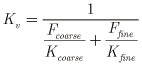 (2)
(2)
where Fcoarse is the fraction of coarse-grained sediment between layer midpoints, and
Ffine is the fraction of fine-grained sediment between layer midpoints.
The calibrated value of Kcorc was 1.3 × 10⁻³ m/d and that for Kfine was 8 × 10⁻³ m/d. The calibrated value of Kcoarse varied by lithologic subarea: 53 m/d for the older fan deposits and 80 m/d for the remaining area. The resulting values of Kh and Kv are summarized in figure 19. The distributions of Kh and Kv are the same as those for the sediment texture (fig. 5).
Effective hydraulic conductivity in the three principal directions of each of 200 texture realizations was estimated using 600 simulations. These simplified simulations were used to compute flow in each principal direction for each realization. Constant-head boundaries were assigned at the up-gradient and down-gradient faces to produce an arbitrary hydraulic gradient of 0.0009, and no stresses were imposed. Isotropic hydraulic conductivities were assigned: 0.08 m/d for the clay hydrofacies, 2 m/d for silt, 24 m/d for silty sand, 160 m/d for sand, and 0.00008 m/d for the Corcoran Clay.
Five of the TProGS-generated realizations of the three-dimensional distribution of hydrofacies within the local model were chosen for calibration and sensitivity. This subset of realizations was selected on the basis of a relative ranking of the bulk flow properties in the X, Y, and Z directions. Four were chosen to represent the extremes:
A fifth realization was chosen randomly for use in developing the local model, and ultimately was used in the calibrated model. Of the 200 realizations, this ranked 54th, 48th, and 33rd for flow in the X, Y, and Z directions, respectively. Figure 20 shows one view of the vertical distribution of hydrofacies for this realization.
To simplify model calibration, the three hydrofacies in the Holocene deposits associated with the incised river channel were assumed to be hydraulically equivalent to the same hydrofacies in the Pleistocene deposits. Therefore, the total remained at four hydrofacies: sand, silty sand, silt, and clay. The overall proportions of these facies are as shown in the Pleistocene section in table 1. The calibrated and specified values of horizontal and vertical hydraulic conductivity associated with each hydrofacies are shown in table 3.
Calibration of the regional model consisted of a systematic application of the parameter estimation method (described in the “Aquifer Hydraulic Properties” section in this report) to narrow the range of possible solutions. This was followed by manual adjustments to best match the highest-quality water-level measurements in midslope areas while simultaneously honoring the overall conditions in upslope and downslope areas. Kcoarse and Kfinewere varied systematically for a given value of Kcorc, which was adjusted to roughly match vertical gradients across the Corcoran Clay (assumed to be isotropic). Simulated hydraulic heads were compared to measured water levels in 49 wells representing various parts of the aquifer system, including 22 wells installed and monitored by the USGS. The resulting error distributions constrained the parameter set and constitute a sensitivity analysis of these parameters.
Wells used to calibrate the regional model were divided into several categories. The first category included the USGS wells and associated measurements, which were considered the highest quality because of the short screened intervals (0.6 to 3 m) and hourly measurements during 2003–2005. Most of these wells are in midslope areas in and near Modesto and the local study area. These wells are multi-depth completions, and thus were used to evaluate simulated vertical gradients as well as simulated hydraulic heads. Two other key categories of wells were defined geographically. The downslope area where the water table is shallow was represented by 17 wells, most of which were 4.6 m deep and monitored on a monthly basis. Data from these wells were ranked second highest in overall quality. The upslope area northeast of Modesto and Turlock was represented by 11 wells, including one USGS well in Eastside Water District. The final well used to calibrate the regional model was a USGS well screened below the Corcoran Clay at the lower end of the USGS well transect in the local study area.
Model error was quantified by average error and the root-mean-square error (RMSE):
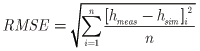 (3)
(3)
where hmeas is measured water level,
hsim is simulated hydraulic head,
i is the summation index, and
n is the number of measurements.
The RMSE is a measure of error magnitude, and average error indicates whether simulated hydraulic heads were, overall, higher or lower than measured water levels. The RMSE and average error calculations were used to estimate the range of Kcoarse and Kfine values that generated parameter distributions with the lowest error for the conceptual model described herein. RMSE and average error values were calculated for 100 simulations at a time, representing progressively narrower ranges of Kcoarse and Kfine. Results from each group of 100 simulations were plotted as error surfaces describing model fit with respect to hydraulic heads for various sets of calibration wells (fig. 21). Each plot in figure 21 shows the error surface for simulated hydraulic heads at the locations of USGS wells or wells representing the upslope and downslope parts of the aquifer system. The model was numerically stable over a wide range of parameter values, but numerical stability decreased as values of Kcoarse and Kfine decreased.
The error surfaces constrain Kcoarse and Kfine to the lower central region of the plot and indicate that relatively high values of Kcoarse and low values of Kfine provide the best solution for the given conceptual model (fig. 21). Simulated values compare well to measurements in the USGS wells, and the error surface defines a zone of minimum error. However, the error surfaces for upslope and downslope areas indicate greater error, no minima near that of the USGS wells, and slope in opposite directions. This indicates there is some error in the conceptual model and (or) the water-level data for the upslope and (or) downslope areas. Subsequent manual calibration efforts focused on matching vertical gradients calculated from measurements in the USGS wells while minimizing error for the downslope wells and key upslope wells and staying within the zone of minimum error for the USGS wells. Results indicate that Kcoarse and Kfine values of about 80 and 8 × 10⁻³ m/d, respectively, generate the best-fit parameter distribution. The associated value of Kcorc (1.3 × 10⁻³ m/d) was adjusted to reasonably match vertical hydraulic gradients calculated from water levels measured in wells screened above and below the Corcoran Clay.
A hydraulic conductivity of 80 m/d is within the typical range of that for clean sand and a hydraulic conductivity of 8 × 10⁻³ m/d is within the range of silty clay (Freeze and Cherry, 1979). Both lithologies are common in the study area and reasonably represent the lithologic end members. Permeameter tests of cores from the Corcoran Clay indicate vertical hydraulic conductivities ranging from 1 × 10⁻⁶ to 3 × 10⁻⁶ m/d (Page, 1977). Previous investigations, however, indicate wells screened across the Corcoran Clay have increased the effective vertical hydraulic conductivity by orders of magnitude by allowing the clay to be short circuited (Williamson and others, 1989; Belitz and Phillips, 1995). The calibrated value of Kcorc from this study (1.3 × 10⁻³ m/d) is consistent with these previous findings. The value estimated by Belitz and Phillips (1995) for an area southwest of the regional model is one order of magnitude lower than that estimated by this study. However, the greater depth of burial of the Corcoran Clay in that area (about 100–240 m) and widespread aquifer-system compaction may have caused a substantial decrease in its vertical hydraulic conductivity.
The simulated water table (fig. 22) resembles the contours of measured water levels depicted in figure 8. A simple method of assessing overall model fit is to plot the simulated head values against the measured water levels. For a perfect fit, all points should fall on the 1:1 diagonal line. Figure 23 is a plot of the simulated heads versus measured water levels for the regional model area and indicates good overall model fit.
Simulated hydraulic heads closely matched measured water levels in USGS wells in the midslope areas, as indicated by an average residual of 0.3 m and a RMSE of 0.8 m. In the downslope area, simulated hydraulic heads in the area underlain by a shallow water table reasonably matched measured heads; the average error was 1.5 m and the RMSE was 3.4 m. Much of this error, and the primary source of the positive average error, was associated with two wells on the northeastern side of this area within Turlock Irrigation District, indicating that the simulated ground-water divide was slightly downslope of the actual divide. Water levels in the upslope area were also simulated well; the average error was 1.2 m and the RMSE was 2.1 m.
The average error for all wells was 0.9 m; the errors ranged from –1.7 to 9.6 m (fig. 22) and the standard deviation was 2.1 m. The associated RMSE was 2.3 m, about 7 percent of the range of head observations in the aforementioned set of wells (32.9 m). The errors for the USGS wells were randomly distributed around zero, and those for the upslope and downslope areas were skewed positive by a few measurements in wells near the ground-water divide and within the cone of depression in the eastern part of the regional study area (fig. 22). Simulated values generally were lower than measured values in these areas, although the error for the only USGS well in Eastside Water District was very small (–0.4 m).
The local model was calibrated using a combination of the Sensitivity and Parameter-Estimation Processes in MODFLOW-2000 (Hill and others, 2000) and manual adjustments. Hourly water-level measurements in 11 USGS wells along a transect north of the Merced River (fig. 11) were averaged on a water-year basis for model calibration. The adequacy of the head-based calibration was evaluated by using computed fluxes to compare simulated and measured concentrations of sulfur hexafluoride, an environmental tracer.
Wells used to calibrate the local model included all 4 at the upper end of the well transect, the 3 deepest wells at the middle site, and 4 wells at the lower end (lower_9, lower_15, lower_25, lower_29) (fig. 3). Hourly water-level measurements were recorded in these wells for 1 to 1.6 years, and annual averages of these measurements were used for model calibration. Data from the shallowest and deepest wells at these sites are shown in figure 11. These well clusters were used to evaluate simulated vertical gradients as well as simulated hydraulic heads.
A subset of the horizontal and vertical hydraulic conductivity values of the four textural categories defined earlier were adjusted during calibration of the local model. Because the model was insensitive to the riverbed conductance, it was not adjusted during calibration. Recharge estimates, the vertical hydraulic conductivity of the Corcoran Clay, and boundary fluxes also were not adjusted during calibration.
The Sensitivity Process in MODFLOW-2000 (Hill and others, 2000) identifies the sensitivity of computed values at the locations of measurements to changes in model parameters. It was used to identify which hydraulic conductivity parameters to include in the Parameter Estimation Process (Hill and others, 2000) and to adjust during subsequent manual calibration. Results of the Sensitivity Process indicate that the local model was most sensitive to the horizontal hydraulic conductivities of the sand, silty sand, and silt hydrofacies, listed here in declining order of sensitivity (fig. 24). The local model was moderately sensitive to the vertical hydraulic conductivity of the clay facies, and essentially insensitive to the remaining hydraulic conductivities. Results also showed that sensitivity was greatest at the upper end of the well transect (fig. 25) because, as in the real system, water levels near the Merced River are controlled primarily by the river stage, not by irrigation.
The most sensitive hydraulic conductivity parameters were estimated initially using the Parameter Estimation Process (Hill and others, 2000), followed by manual adjustments. The Parameter Estimation Process minimizes a weighted least-squares objective function, thereby finding the optimal solution to the problem, assuming it converges numerically. The average water levels used as observations were not weighted, because identical equipment and methods were used to derive the measurements. The Parameter Estimation Process did not converge for this model, but did approach the optimal solution prior to diverging. Parameter estimation fit the water levels well, but not the vertical gradients. Hydraulic properties were adjusted manually to better match vertical gradients, which were not explicitly included in the objective function.
The calibrated hydraulic conductivity values for the local model (table 3) can be compared to values for a wide range of sedimentary materials and to the results from slug tests of local materials. A hydraulic conductivity of 80 m/d is within the range typical for clean sand, and 30 m/d is within the range for silty sand (Freeze and Cherry, 1979). Slug tests were done in 18 wells in the bed and on the banks of the Merced River down-gradient of the well transect (Zamora, 2006). The sediments tested ranged from silty sand to well-sorted coarse sand, and computed hydraulic conductivity values ranged from 15 to 250 m/d; the mean value was 85 m/d. These values are consistent with those derived by calibrating the local model.
Both hydraulic conductivity estimates for the coarsest fraction above the Corcoran Clay in the local and regional models were 80 m/d. The local calibrated value for the vertical hydraulic conductivity of clay (0.15 m/d), however, was about an order of magnitude greater than the vertical hydraulic conductivity above the Corcoran Clay in the regional model (median of 0.012 m/d). Simulated vertical hydraulic gradients in the regional model within the local study area (fig. 22) were greater than those measured, suggesting that spatial variability exists in the vertical hydraulic conductivity of fine-grained materials. Lower values for the vertical hydraulic conductivity of clay in the local model increased vertical gradients above those calculated from average measured water levels, which were very small (absolute value of about 0–0.02).
figure 26 is a plot of the simulated hydraulic heads versus measured water levels for the local model and indicates excellent model fit. Average water-level measurements from 11 USGS transect wells were very closely simulated; the average error was 0.0 m and the RMSE was 0.08 m. Errors ranged from –0.3 to 0.16 m; the standard deviation was 0.17 m. The RMSE was less than 2 percent of the range of head observations in the 11 wells (4.4 m). The largest errors were at the middle site of the transect, ranging from 0.3 m near the water table (well middle_13) to 0.23 m at the deepest well (middle_25). All simulated heads at the middle site were greater than measured water levels. Errors at all other transect wells were less than 0.16 m. The simulated water table is shown in figure 27.
Calibration of a model to hydraulic heads alone generally results in a non-unique set of parameters. Other parameter sets may generate roughly the same head distribution, but simulated fluxes would vary; therefore, it is useful to evaluate head-based calibrations using some measure of system flux. An environmental tracer, sulfur hexafluoride, was used to evaluate the fluxes in the calibrated local model. Areal recharge and boundary fluxes were specified in the local model, and consequently the internal fluxes were highly constrained. Thus, the following analysis was more effective in this case as a check on the specified fluxes than as a means for evaluating hydraulic parameters.
Samples collected from most of the USGS wells along the transect in the local study area were analyzed for sulfur hexafluoride (SF6), generally a non-reactive, conservative environmental tracer in ground water (Busenberg and Plummer, 2000). Atmospheric concentrations of SF6 were very low prior to 1965 and have increased since then, making it a good means of dating young ground water. Particle-tracking software, MODPATH (Pollock, 1994), was used in conjunction with flux output from the local flow model to calculate backward flow paths and associated travel times for water particles traveling back in time from the screened intervals of sampled wells to the water table. The travel time for each particle (64 per well screen, represented by one model cell) represented only the advective component of flow, but included the effects of macro-scale mechanical dispersion caused by the three-dimensional distribution of hydrofacies.
Effective porosity was the only hydraulic parameter specified in the MODPATH input files. Effective porosity values were assigned on the basis of the hydrofacies represented by each model cell. Sand, silty sand, silt, and clay were assigned effective porosities of 0.3, 0.35, 0.38, and 0.4, respectively. These porosity values were based on literature values for different geologic/textural materials (Domenico and Schwartz, 1990), previous studies of similar geologic formations in the eastern San Joaquin Valley (Burow and others, 1999), and measurements made using sediment cores collected during the installation of the transect wells. Four cores that averaged 89 percent sand had moisture contents ranging from 32 to 37 percent, and a single core consisting of 83 percent silt had a moisture content of 48 percent. Effective porosity is a lower value than moisture content, and the difference between them increases with increasing content of fine-grained materials; thus, the estimated effective porosities are consistent with those measured in the local study area.
The travel time for each particle was used to determine the atmospheric concentration of SF6 when the particle was at the water table. Assuming conservative transport and steady-state conditions, the average atmospheric concentration of SF6 associated with all particles for a given well screen can be compared with the measured concentration in the well (table 4). Simulated concentrations at or near the water table are higher (younger age) than those measured at all sites, but concentrations at depth generally compare well. The cause of the disparity in shallow concentrations is unknown, but the good agreement between simulated and measured SF6 concentrations deeper in the system suggests that fluxes, which are largely controlled by specified recharge and boundary conditions, are reasonably simulated.
The calibrated hydraulic conductivities for the local model (table 3) were based on one of 200 realizations of the three-dimensional distribution of hydrofacies. The sensitivity of parameters to their distribution was determined using four end-member realizations. These end members represented the minimum and maximum effective three-dimensional hydraulic conductivity and domain-scale vertical anisotropy. Each realization was upscaled into the regional model, which was then used to generate a new set of specified fluxes for the lateral boundaries of the local model. The local model, with each realization incorporated, was then re-calibrated until the total error approached that of the calibrated model, if feasible. Generally, this was accomplished through changes in only the most sensitive horizontal (sand) and vertical (clay) hydraulic conductivities.
The sensitivity of key hydraulic conductivity parameter estimates to the three-dimensional distribution of hydraulic conductivity is shown in table 5. All but one realization required adjustment of only the horizontal hydraulic conductivity of sand to achieve nearly the same error as the calibrated model. These adjustments ranged from a reduction of 25 percent to an increase of 12.5 percent. The realization representing minimum domain-scale vertical anisotropy required a threefold decrease in the vertical hydraulic conductivity of clay and was associated with relatively high error. Adjustments of other hydraulic conductivity values failed to reduce the error for this realization, suggesting that model performance decreases below a minimum threshold for vertical anisotropy. This analysis indicates that if this threshold is met, the overall sensitivity of hydraulic conductivity parameter estimates to the distribution of hydrofacies is fairly low.
The sensitivity of parameter estimates for the local model to areal recharge was determined by increasing and reducing recharge by 20 percent, a quantity that would represent substantial error in the water budget. The local model was re-calibrated by adjusting the horizontal hydraulic conductivity of sand and vertical hydraulic conductivity of clay, achieving a total error within 13 percent of that of the calibrated model. Reducing recharge by 20 percent required a 50-percent reduction in the conductivity of sand. A 20-percent increase in recharge required increasing the hydraulic conductivity of sand by 38 percent and doubling the hydraulic conductivity of clay. This analysis shows that the sensitivity of hydraulic parameter estimates to large changes in areal recharge, which represents 76 percent of the total recharge, is moderate.
The effects of changes in the hydrofacies distribution and areal recharge rates on the simulated water budget were straightforward. Small changes in net boundary fluxes related to hydrofacies distribution, and large changes in areal recharge rates, were balanced by like changes in discharge to the Merced River.
The simulated water budget for the regional-scale model is presented in table 6. Note that many of the water-budget components of the regional model were specified values. Areal recharge was mostly agricultural irrigation and precipitation, accounting for 80 percent of the total recharge; urban recharge added another 1 percent to the total. Areal recharge estimates were reduced from those of Burow and others (2004) by 10 percent during calibration, but remain the dominant component of recharge. Leakage from reservoirs contributed about 4 percent of the recharge, and the rivers less than 1 percent (net). Pumpage from wells, primarily for agriculture, was about 70 percent of the total discharge. About 6 percent of the discharge was bare-soil evaporation from the shallow water table. The remainder of the simulated water budget was flow through the lateral head-dependent boundaries, which was about a net 8-percent export.
Flow through the lateral boundaries is different at each boundary. The northern boundary is dominated by northward flow above and below the Corcoran Clay, exiting the regional study area. This is consistent with the limited available water-level data for the area north of the Stanislaus River (fig. 8). This northward flow is 13 percent of the simulated budget, more than twice the flow at any other lateral boundary. The southern boundary is characterized by flow entering the regional model and moving toward the Merced River above the Corcoran Clay, and exiting below the clay and at depth east of the clay. Flow is in the opposite sense along the western boundary, exiting the model area above the Corcoran Clay, and entering from below. The southern boundary and the western boundary each have a simulated net flux into the regional model domain that comprises only 1–2 percent of the total water budget.
The simulated water budget for the local-scale model is given in table 7. Note that most of the water-budget components of the local model were specified values. Areal recharge, which was dominated by agricultural irrigation and precipitation, accounted for 76 percent of the total recharge. Discharge was dominated by flow to the Merced River (65 percent), and included downward flow through the Corcoran Clay (16 percent). The remainder of the simulated water budget was flow through the lateral specified-flux boundaries, which was a net 5-percentage gain.
The dominance of areal recharge and discharge to the Merced River results in downward flow in most of the local study area and upward flow along the Merced River, which is consistent with measured water levels along the well transect. This flow configuration, coupled with downward flow through the Corcoran Clay, results in primarily locally-recharged ground water discharging to the Merced River. The combination of measured sulfur hexafluoride concentrations and travel times of simulated particles (table 4) suggests that most of the ground water discharging to the Merced River was recharged less than 25 years ago.
The regional and local ground-water flow models were developed to generate a better understanding of the flow system at both scales. The local model will be used to help understand the transport and fate of agricultural chemicals in the local study area. Limitations of the modeling software, assumptions made during model development, and results of model calibration and sensitivity analysis all are factors that constrain the appropriate use of these models and highlight potential future improvements.
A ground-water flow model is a means for testing a conceptual understanding of a system. Because ground-water flow systems are inherently complex, simplifying assumptions were made in developing and applying model codes (Anderson and Woessner, 1992). Models solve for average conditions within each cell, the parameters for which are interpolated or extrapolated from measurements, and (or) estimated during calibration. In light of this, the intent in developing the regional and local ground-water flow models was not to reproduce every detail of the natural system, but to portray its general characteristics. Results from these models should be interpreted generally and are best suited for comparative analysis rather than for prediction.
A steady-state model portrays a system that is in equilibrium. Although water-level hydrographs suggest this generally was the case in the regional study area for the year 2000 (fig. 9), the data were not conclusive. Long-term hydrographs are not available for some areas, including the southeastern part of the model area, where hydraulic heads may have been changing with time. There are no long-term water-level records available in the local model area, but the closest wells show little change in about 40 years of record. Errors related to the assumption of a steady-state condition may be significant in places, and care must be taken in interpreting model results and analyses that depend on model output, including particle tracking.
A problem related to the steady-state assumption for both models was that stresses were based on data from water year 2000, but the water levels for USGS wells were measured during 2003–2005. Although this may be a source of model error, none of these years represented climatic aberrations. It is likely that deliveries of surface water for agricultural and urban use, and associated ground-water pumpage, varied little during these years.
Some of the boundary conditions of the regional model were poorly constrained, which may be a source of model error. The western and northern lateral boundaries were based on sparse data; the spatial distribution of hydraulic head below the river was poorly understood, and there were no available data in the western part of the northern area. Similarly, there was little regional information on river-aquifer interaction and the hydraulic conductivity of riverbed sediments. Simulation results indicated that flows across these poorly constrained boundaries (table 6) generally made up a small part of the water budget; however, this may not be true in the real system.
The accuracy of model results is related strongly to the quality and spatial distribution of input data and of measurements of system state (for example, measured water levels) used to constrain the calibration. The local study area and the Modesto area were the only locations in the regional model that had high-quality input data, including pumpage by well and sediment texture, coupled with a good distribution of high-quality water-level measurements. The stresses in other areas of the model were a combination of measured values and values estimated from the water-budget analysis. Accordingly, the user should have more confidence in simulation results in the local study area and the Modesto area than in other parts of the model.
The regional estimate of the vertical hydraulic conductivity of fine-grained materials was about one order of magnitude lower than that estimated at the local scale. Simulated vertical hydraulic gradients are more accurate (smaller) in the local model than in the regional model within the local study area (figs. 27, 22). This suggests that there may be substantial spatial variability in the vertical hydraulic conductivity of fine-grained materials that is not accounted for in the regional model.
The specified areal recharge and lateral boundary conditions in the local model, which account for all of the simulated recharge, highly constrain the internal fluxes. This, in turn, constrains the range of estimated hydraulic conductivities. Key hydraulic conductivity values are sensitive to substantial changes in areal recharge; rates of chemical transport are expected to be equally sensitive. In contrast, these key hydraulic conductivity values, and associated fluxes, are less sensitive to the three-dimensional distribution of the four defined hydrofacies.
All of the water-level data used to calibrate the local model were collected from USGS transect wells, which are concentrated in the central part of the model domain. Accordingly, the user should have higher confidence in simulation results for the area near the well transect than for other areas represented in the model.

![]() U.S.
Department of the Interior | U.S. Geological Survey
U.S.
Department of the Interior | U.S. Geological Survey
Persistent URL: https://pubs.water.usgs.gov/sir20075009
Page Contact Information: Publications Team
Page Last Modified: Thursday, 01-Dec-2016 19:40:17 EST
