Scientific Investigations Report 2007–5044
U.S. GEOLOGICAL SURVEY
Scientific Investigations Report 2007–5044
Model calibration is the adjustment of model parameters (such as hydraulic conductivity and specific yield) so that the differences between simulated and measured quantities (such as water levels and flows) are minimized with respect to an objection function. This section of the report describes the nonlinear least-squares regression method used for calibration, the calibration data, and the calibration results. The calibration is assessed by examining how well the simulated quantities fit the measured quantities. Model assumptions are examined by comparing the calibrated model with several alternative models.
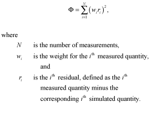
The parameter estimation program PEST version 10 (Doherty, 2004) is used to calibrate the SVRP aquifer model. PEST implements a nonlinear least-squares regression method to estimate model parameters by minimizing the sum of squared weighted residuals:
 (9)
(9)
The sum of squared weighted residuals, Φ, also is known as the objective function. PEST uses the Gauss-Marquardt-Levenberg method to minimize Φ. Details of this method are given in the PEST user’s manual (Doherty, 2004).
The weight, wi, reflects the importance of the ith measured quantity on the regression. A measurement with a large wi asserts a large influence on the regression and, therefore, the estimated parameter values. Conversely, a measurement with a small wi asserts a small influence on the regression and estimated parameter values. Note that the notation for wi follows the convention used in the PEST manual. Other authors (for example, Hill, 1998) express equation 9 as
 (10)
(10)
and define ωi as the weight. Therefore, wi as used in this report is equivalent to the square root of ωi in equation 10.
The SVRP aquifer model is calibrated using both water-level and flow measurements. Water-level measurements include:
A total of 1,573 water-level measurements are used in the model calibration. Water-level measurements for several wells are excluded as calibration data. A well is excluded if it meets one of the following criteria: (a) the well is completed in bedrock or in both bedrock and in aquifer sediments, (b) the well encounters the narrow ground-water mound beneath the losing segment of the Spokane River upstream of the gaging station at Greenacres, and (c) the well is located along the aquifer boundary where water levels differ by more than several tens of feet from those of nearby wells.
Flow measurements consist of streamflow gains and losses along segments of the Spokane and Little Spokane Rivers. Flow measurements include:
A total of 313 flow measurements are used in the model calibration.
A standard approach to determining the weight for a measured quantity is to calculate wi as the inverse of the standard deviation of the error associated with the ith measured quantity (Hill, 1998). To apply this approach, the following sources of error are evaluated for water-level measurements:
Following Hill’s (1998, p. 46) suggestion, each of the above error values is interpreted as a 95-percent confidence interval. For example, a land-surface datum error of 10 ft is interpreted to mean that the probability is 95 percent that the actual land-surface datum is within ±10 ft of the measured datum. If the error is assumed to be a normally distributed random variable, then a 10-ft error is equal to 1.96 times the standard deviation. Therefore, the standard deviation is 5.1 ft. To account for multiple sources of errors, the variance (square of standard deviation) for each error source is computed, the variances are summed, and the square root of the sum is calculated. This gives the standard deviation of the total error. The weight then is computed as the inverse of this standard deviation.
A similar procedure (Hill, 1998, p. 46-47) is used to determine the weights of the flow measurements (streamflow gains and losses). Because the streamflow gain or loss on a river segment is determined from the difference between streamflows at the upstream and downstream ends of the river segment, the variances of the errors of the two streamflow values are summed. Based on the study by Sauer and Meyer (1992), the error of a streamflow measurement is estimated to be 5 percent of the measured value. To illustrate the weight calculation, suppose the streamflow at the upstream gaging station is 1,000 ft3/s and the streamflow at the downstream gaging station is 800 ft3/s, giving a streamflow loss of 200 ft3/s. For the streamflow at the upstream gaging station, the error is 50 ft3/s. Interpreting this error to equal 1.96 times the standard deviation gives a standard deviation of 25.5 ft3/s, or a variance of 651 (ft3/s)2. By the same reasoning, the error of the streamflow at the downstream gaging station is 40 ft3/s, giving a standard deviation of 20.4 ft3/s and a variance of 416 (ft3/s)2. The variance of the error of the streamflow loss (200 ft3/s) is the sum of the variances of the upstream and downstream streamflows, or 1,067 (ft3/s)2. The standard deviation is 32.7 ft3/s, and the weight is the inverse of the standard deviation.
Initial calibration runs using weights determined by the previously described procedure indicated that the sum of squares of weighted residuals is heavily dominated by the water-level measurements, and the fit to flow measurements is poor. This results from the fact that (1) the number of water-level measurements is five times the number of flow measurements, and (2) relative errors in water-level measurements generally are much smaller than relative errors in flow measurements. To create a more even balance between the weighted water-level residuals and the weighted flow residuals, the weights for water-level measurements are reduced by adding 5 ft to the standard deviations of the water-level errors. This adjustment improves the fit to flow measurements without substantially degrading the fit to water-level measurements.
The calibration set-up as previously described involves 42 parameters. These parameters are listed in the first column of table 8. During the initial calibration phase, it was determined that calibration data were insensitive to HK1-21 (the horizontal hydraulic conductivity of the side valley in which Newman Lake is located) and KVSR-11 (the vertical hydraulic conductivity of the streambed sediments in the segment of the Spokane River in the Little Spokane River Arm). In addition, initial calibration runs yielded relatively high values of C-OUT (the boundary conductance for outflow from the lower unit to Long Lake), but the estimated C-OUT was nonunique and varied from one calibration run to another depending on starting parameter values. In addition, the estimated value of HK3-2 (horizontal hydraulic conductivity of the lower unit in the Little Spokane Arm) was unreasonably high. Therefore, the four previously mentioned parameters are not estimated by calibration but are assigned as follows. HK1-21 is set to 150 ft/d. This Kh value results in a simulated water level of about 2,100 ft in the vicinity of Newman Lake. This water level is about 30 ft below the level of Newman Lake. KVSR-11 is set to 0.1 ft/d. This Kv value limits the interaction between the aquifer and the segment of the Spokane River in the Little Spokane River Arm. The limited interaction is reasonable because most of the ground-water discharge in the Little Spokane River Arm would enter the Little Spokane River. C-OUT is set to a relatively high value of 106 ft2/d. Increasing or decreasing this value by one order of magnitude has little or no effect on the simulation results. However, setting a high value for C-OUT is nearly equivalent to setting the head at the outflow boundary close to the level of Long Lake. HK3-2 is set to 2,000 ft/d. This value based on Kh values estimated for the Hillyard Trough area (see fig. 6).
The PEST program requires specifying an acceptable interval for each estimated parameter. The lower and upper limits defining this interval are given in the third and fourth columns of table 8. For hydraulic conductivity and conductance, the acceptable interval is set fairly wide, with the expectation that the estimated value would fall within the acceptable interval. For specific yield, the acceptable interval is set from 0.1 to 0.3. PEST always yields an estimated value that is within the parameter’s acceptable interval (inclusive of the upper and lower limits).
Estimated values obtained from the calibration are given in the fifth column of table 8. A value in bold indicates that the estimated value is at either the upper or lower limit of the acceptable interval. In the central part of the aquifer in Rathdrum Prairie and in Spokane Valley, estimated Kh values ranged from 6,170 to 22,100 ft/d. In Hillyard Trough, the Little Spokane River Arm, and Western Arm, estimated Kh values ranged from 1,980 to 3,110 ft/d. In the Coeur d’Alene area, the estimated Kh value is 1,290 ft/d. For side valleys and regions of shallow bedrock along the margins of the aquifer, estimated Kh values ranged from 5 to 140 ft/d. These estimated Kh values generally are consistent with Kh values estimated in previous studies (see the discussion in the section, “Hydraulic Properties.”).
Estimated SY values are 0.1 for SY-1, 0.19 for SY-2, and 0.21 for SY-3. The estimated SY-1 value is at the lower limit of the acceptable range. The implication of this calibration result is explored using alternative model C in the section, “Alternative Models.”
Estimated Kv values of streambed sediments indicate that these parameters are related to gaining and losing segments of the Spokane River. Along losing segments of the Spokane River, estimated Kv values of streambed sediments are less than 1 ft/d (parameters KVSR-1 to KVSR-4, KVSR-6, and KVSR-8). Along gaining segments of the Spokane River, estimated Kv values of streambed sediments are greater than 1 ft/d (parameters KVSR-5, KVSR-7, KVSR-9, and KVSR-10). These results support the suggestion by Caldwell and Bowers (2003) that the transport of fine-grained material with the leaking water from the Spokane River might decrease Kv of the streambed sediments along a losing segment of the river.
The sixth and seventh columns of table 8 give the linear, 95-percent confidence interval for the estimated parameter values. These confidence intervals should be interpreted with caution. The confidence intervals are approximate and are computed under the assumption that the model is linear with respect to the parameters in the vicinity of the estimated values. If this linearity assumption is not valid, then the confidence intervals are inaccurate.
The results of the calibration can be assessed by comparing simulated and measured quantities and by examining the weighted residuals. Simulated and measured water levels in selected wells in various parts of the SVRP aquifer are shown in figure 41. Except as noted, the same scale is used for all vertical axes for ease of comparison of water-level fluctuations in different wells.
For the upgradient end of the aquifer near Lake Pend Oreille, simulated and measured water levels in well 236 are in close agreement (fig. 41A). For northern Rathdrum Prairie, simulated and measured water levels in well 251 (fig. 41B) and well 249 (fig. 41C) are compared. In well 251, the simulated rise in water level during 1996 and 1997 is not as large as the measured rise. In both wells 249 and 251, the simulated fluctuations during 2004 and 2005 are somewhat larger in magnitude than the measured fluctuations. These discrepancies likely are due to two simplifying assumptions used in calculating recharge from precipitation: (1) use of a triangular network to linearly interpolate recharge from precipitation (fig. 7), and (2) use of a linear relation between depth of water table and transmission time for precipitation infiltration to reach water table (table 2).
For southern Rathdrum Prairie, simulated and measured water levels in well 225 (fig. 41D) and well 178 (fig. 41E) are compared. In both wells, the simulated water levels are close to the measured water levels, but the character of the simulated fluctuations during 2004–05 does not match the character of the measured fluctuations. The same discrepancy is shown in the simulated and measured water levels in well 143 (fig. 41F), which is near Coeur d’Alene Lake. These discrepancies indicate that the temporal distribution of recharge to southern Rathdrum Prairie (including the Coeur d’Alene area) might not be represented accurately in the model for 2004–05.
Simulated and measured water levels in well 246 near the east edge of Rathdrum Prairie and in well 140 in a side valley between Coeur d’Alene and Hayden are shown in figures 41G and 41H, respectively. Note that the vertical axes in both figures span 120 ft. Although these wells have few long-term historical data for calibration, the simulation indicates that water levels along the margins of Rathdrum Prairie can rise and decline by substantial amounts.
Simulated and measured water levels in wells in various parts of Spokane Valley are shown in figures 41I to 41M. Overall, the seasonal rise and decline of simulated water levels reproduce the measured water levels. However, simulated fluctuations on short time scales do not always match the measured fluctuations. For example, each year during September, the measured water level in well 92 (fig. 41K) rises in response to the rise in Spokane River stage as the gates at the Post Falls Dam are opened. However, the simulated water level during September does not always follow the rises in the measured water level. This discrepancy might be a consequence of assuming a rectangular cross-section for the channel of the Spokane River. Under this assumption, the streambed area through which seepage occurs is independent of river stage. In reality, under low-flow conditions typical of later summer, the river might occupy only a portion of the streambed. As the river stage rises in September, the river might occupy a larger area of streambed. Because the model does not simulate this increase in wetted streambed area, the simulated exchange between the aquifer and the Spokane River might be inaccurate during early autumn.
Simulated and measured water levels in well 6 in Trinity Trough are shown in figure 41N. The magnitude of the simulated water-level fluctuation is substantially smaller than the magnitude of the measured fluctuation. During 2004–05, the water level in well 6 rose and declined by about 15 ft. This is nearly double the magnitude of the fluctuations in other wells in Spokane Valley. Well 6 is located in an area of steep hydraulic gradient as ground water is channeled through Trinity Trough into Western Arm (fig. 22). The discrepancy between simulated and measured water levels in well 6 might indicate that a finer model grid (with smaller model cells) is needed to more accurately represent Trinity Trough.
Simulated and measured water levels in well 128 in Hillyard Trough and in well 107 in Western Arm are shown in figures 41O and 41P, respectively. For both wells, the simulated water levels are in fairly good agreement with the measured water levels.
Simulated and measured water levels in the lower unit are shown in figures 41Q and 41R. Well 115 (fig. 41Q) is at the north end of Hillyard Trough. The drawdowns during 2004–05 are a result of pumping of a nearby production well. However, the simulated drawdowns were substantially larger than the measured drawdowns, indicating that the estimated value of KH3-1 might be too low. Well 99 (fig. 41R) is located on the west side of the Little Spokane River Arm. In this well, simulated water levels were about 15 ft higher than the measured water levels. Considered together, the relatively poor fits to measured water levels in wells 115 and 99 indicate that the lower unit might not be represented accurately by the model.
Simulated water levels in model layer 1 during September 2004 are shown in figure 42. The contours of simulated water levels shown in figure 42 are in good agreement with the contours of measured water levels shown in figure 22. Simulated water levels in model layer 3 during September 2004 are shown in figure 43. Because water-level measurements are available for only two wells in the lower unit, too few data are available to construct a map of measured water levels in the lower unit.
Simulated and measured monthly average streamflow gains and losses for the Spokane River segments from the gaging stations near Post Falls to at Spokane, near Post Falls to at Greenacres, and at Greenacres to at Spokane are shown in figure 44. The length of the vertical line extending above or below a plotted point indicates the measurement error, calculated as 1.96 times the standard deviation used in the calculation of measurement weights. During times of high streamflow (winter and spring), measurement errors can be very large. The simulated streamflow gains and losses generally agree with the measured gains and losses during late summer, when streamflow is low and the measurement error is small.
For the Spokane River segment from the gaging stations near Post Falls to at Greenacres (fig. 44B), data show a decrease in the magnitude of streamflow loss during the first halves of 2003 and 2004 when the river stage is high. This is an unexpected phenomenon because the altitude of the bottom of the riverbed from the gaging stations near Post Falls to at Greenacres is always above the water table. Therefore, the magnitude of streamflow loss is expected to increase (as indicated by the simulated quantity) during winter and spring when the river stage is high. If the measured streamflow at the gaging station at Greenacres is inaccurate (too low) during the first halves of 2003 and 2004, the error might account for the poorer fit during the same two periods for the segment from gaging stations at Greenacres to at Spokane (fig. 44C).
The simulated and measured monthly average streamflow gains on the Little Spokane River from the gaging stations at Dartford to near Dartford are in overall agreement as shown in figure 45. The simulated streamflow gain represents the regional discharge from the SVRP aquifer and is remarkably constant. The measured streamflow gain exhibits fluctuations during winter and spring. Nonetheless, the simulated gains are within the error bounds of the measured gains.
Simulated and measured streamflow gains and losses on various Spokane River segments during the seepage runs of September 13-16, 2004, and August 26-31, 2005, are shown in figure 46. The measurements made during the seepage runs might be characterized as nearly instantaneous. By contrast, the simulated streamflow gains and losses represent quantities averaged over a stress period (1 month). Nonetheless, the simulated and measured quantities are in relatively good agreement.
Simulated and measured streamflow gains and losses on three Little Spokane River segments during the seepage runs of September 13-16, 2004, and August 26-31, 2005, are shown in figure 47. The simulated streamflow gains and losses are close to the measured streamflow gains and losses except for the river segment from the gaging station near Dartford to the streamflow measurement site near the mouth of the river. For this segment, the data indicate a small streamflow loss. As discussed previously, this Little Spokane River is not expected to lose streamflow in the Little Spokane River Arm of the SVRP aquifer because this is an area of ground-water discharge. The calibrated model simulates essentially no interaction between the aquifer and this segment of the Little Spokane River.
The spatial distribution of weighted water-level residuals in model layer 1 during September 2004 is shown in figure 48. Ideally, weighted residuals should be distributed randomly throughout the model area. In figure 48, however, the positive weighted residuals tend to cluster locally with other positive weighted residuals, and the negative weighted residuals tend to cluster locally with other negative weighted residuals. The clustering likely is caused by the representation of aquifer properties by zones of uniform values. This simplification might be considered a source of model error in the sense that such error can be reduced by implementing a more complex distribution of aquifer properties in the model. Nonetheless, zonation is widely accepted as a useful approach for model calibration. Although the spatial distribution of weighted residuals shown in figure 48 cannot be characterized as an ideal distribution, the distribution does not show signs of gross model errors over large parts of the aquifer.
The weighted water-level residuals and simulated water levels are shown in figure 49. The plotted points show a fairly random distribution of weighted residuals above and below zero for all simulated water levels. This feature indicates that the simulated water levels fit measured water levels as well in an upgradient region (such as northern Rathdrum Prairie) as in a downgradient region (such as Western Arm). Similarly, the plotted points for weighted flow residuals and simulated streamflow gains and losses (fig. 50) show a fairly random distribution of points above and below zero for all simulated quantities. This feature indicates that the simulated flows fit the measured flows as well in a gaining river segment as in a losing river segment. The vertical band of points shown in figure 50 corresponds to weighted flow residuals for the Little Spokane River. The cluster pattern results from the fact that simulated streamflow gains on the Little Spokane River are relatively constant over time whereas the measured streamflow gains show fluctuations during the winter and spring (fig. 45).
To examine simulated ground-water movement, the SVRP aquifer is divided into eight subregions, seven of which are shown in figure 51. The eighth subregion is the lower unit, which underlies Hillyard Trough and the Little Spokane River Arm. For each subregion, simulated inflows, outflows, and change in storage are averaged over the model calibration period from October 1995 to September 2005 and are given under the Calibrated Model column in table 9. Additional columns in table 9 contain water-budget components for alternative models discussed in the next section of this report. Note that quantities averaged over the 10-year calibration period have slightly different values than the corresponding 15-year averaged quantities given in the sections, “Inflows to Aquifer” and “Outflows from Aquifer”.
For each subregion, inflow components include recharge from precipitation, flow from tributary basins, flow from lakes and losing segments of rivers, and flow from the upstream subregion. Outflow components include net water use (well withdrawals minus return percolation from irrigation and effluent from septic systems), flow to gaining segments of rivers, and flow to the downstream subregion.
Many of the flow components in the subregional water budget are specified in the model. These components are shown in italic and include recharge from precipitation, net water use, and flow to the aquifer from tributary basins and from all lakes except Lake Pend Oreille and Coeur d’Alene Lake. In addition, the model is calibrated to fit measured flows between the aquifer and the Spokane and Little Spokane Rivers. Therefore, the flow components that are neither specified nor constrained by calibration data are: (1) inflow to the aquifer from Lake Pend Oreille, (2) inflow to the aquifer from Coeur d’Alene Lake, and (3) outflow from the aquifer (lower unit) to Long Lake. The calibrated model gives a 10-year average flow of 67 ft3/s from Lake Pend Oreille to the aquifer, 138 ft3/s from Coeur d’Alene Lake to the aquifer, and 27 ft3/s from the lower unit to Long Lake.
On the east side of the aquifer, flow from a subregion to the adjacent downgradient subregion increases along the direction of ground-water flow. The simulated 10-year average flow from northern Rathdrum Prairie to southern Rathdrum Prairie is 286 ft3/s, of which 72 percent flows through West Channel, 26 percent flows through Ramsey Channel, and 2 percent flows through Chilco Channel (table 9, fig. 51). The simulated 10-year average flow from southern Rathdrum Prairie to eastern Spokane Valley is 823 ft3/s. The boundary between eastern Spokane Valley and the Spokane area coincides with Sullivan Road, which crosses the Spokane River near the point where the river changes from a losing stream to a gaining stream. The simulated 10-year average flow from eastern Spokane Valley to the Spokane area is 1,280 ft3/s.
From the Spokane area, the simulated 10-year average outflows are 623 ft3/s to the Spokane River, 288 ft3/s to Hillyard Trough, and 264 ft3/s through Trinity Trough to Western Arm. From Hillyard Trough, the simulated 10-year average outflows are 254 ft3/s to the upper unit in Little Spokane River Arm (and eventually to the Little Spokane River) and 27 ft3/s to the lower unit (and eventually to Long Lake).
To examine the assumptions in the SVRP aquifer model, five alternative models are analyzed. In each alternative model, one aspect of the calibrated model is modified and the alternative model is recalibrated. Estimated values of parameters and regression statistics from the calibrated and alternative models are given in tables 10 and 11.
In alternative model A, the value of HK1-15 (Kh of the zone next to Coeur d’Alene Lake) is set to 500 ft/d (table 9). This value is similar to the hydraulic conductivity value used in Sagstad’s (1977) Darcy’s Law calculation of seepage from Coeur d’Alene Lake (see section, “Lakebed Seepage and Surface Overflow”). In the calibrated model, the value of HK1-15 is 1,290 ft/d and the simulated 10-year average seepage from Coeur d’Alene Lake is 138 ft3/s. Using a lower value of HK1-15 in alternative model A effectively limits the seepage from Coeur d’Alene Lake. Compared to the calibrated model, alternative model A has higher Kh values in northern Rathdrum Prairie (HK1-1, HK1-2, and HK1-3) and a lower conductance value for the Coeur d’Alene lakebed sediments (C-CDA) (table 10). The simulated 10-year average seepage from Lake Pend Oreille to the aquifer increases to 107 ft3/s (table 9), and the simulated 10-year average seepage from Coeur d’Alene Lake to the aquifer decreases to 29 ft3/s, which is close to Sagstad’s (1977) estimated of 37 ft3/s. However, as shown in table 11, the sum of squared weighted residuals from alternative model A is only about 1 percent higher than that from the calibrated model. This indicates that the simulated quantities from alternative model A fit the measured quantities nearly as well as the simulated quantities from the calibrated model.
In alternative model B, the value of HK3-2 (Kh values for the lower unit in the Little Spokane River Arm) is not specified but is estimated. The calibration yields an HK3-2 value of 7,030 ft/d (table 10). The simulated 10-year average flow from the lower unit to Long Lake increases to 83 ft3/d (table 9). The sum of squared weighted residuals decreases to less than that of the calibrated model, indicating an improved fit to measured water levels in wells 99 and 115. However, this improved fit is attained at the cost of allowing HK3-2 to take on a value substantially higher than the upper limit of the acceptable range for this parameter. The occurrence of this trade-off is an additional indication that the model might not accurately represent the lower unit.
In alternative model C, the lower limit of the acceptable range for SY-1 is decreased from 0.1 to 0. In this case, the calibration yields an SY-1 value of 0.08 (table 10). However, the estimated values and the regression statistics from alternative model C are very close to those from the calibrated model (table 9 and 11). This indicates that setting a lower limit of 0.1 for SY-1 results in just as good a fit as allowing SY-1 to take on an estimated value less than 0.1.
In alternative model D, an inflow of 40 ft3/s is applied to the model boundary near Spirit and Hoodoo Valleys (boundary segment A-B in fig. 2). In the calibrated model, there is no inflow across this boundary segment to the aquifer. Compared to the calibrated model, alternative model D has higher Kh values in northern Rathdrum Prairie (HK1-1, HK1-2, and HK1-3) (table 10). The simulated 10-year average seepages are 95 ft3/s from Lake Pend Oreille and 104 ft3/s from Coeur d’Alene Lake (table 9). As in alternative model A, the sum of squared weighted residuals from alternative model D is just slightly higher than that from the calibrated model (table 11). This indicates that amount of inflow from the model boundary near Spirit and Hoodoo Valleys cannot be determined reliably from calibration of the SVRP aquifer model with the present calibration data.
Alternative model E is a hybrid calibration that consists of a steady-state model in additional to the transient model. The steady-state model simulates average conditions for water year 2005 (October 2004 through September 2005). Simulated water levels and flows from the steady-state model are fitted to averages of water levels and flows measured during water year 2005. The purpose of simultaneously calibrating a transient and a steady-state model is to examine the use of the SVRP aquifer model for steady-state simulations.
In general, a steady-state model can be used to simulate average conditions over a period (for example, one year) if (1) heads throughout the aquifer at the beginning of the period are similar to the heads at the end of the period and (2) the model is linear or nearly linear with respect to head. Because the SVRP aquifer is a water-table aquifer, nonlinearity can occur along the aquifer margins, where saturated thickness is small. To avoid such nonlinearity, measured water levels along the aquifer margins are excluded from the steady-state calibration data, with the understanding that the steady-state model might not accurately simulate water levels along the aquifer margins.
The sum of squared weighted residuals from alternative model E is higher than that from the calibrated model (table 11), because the hybrid calibration involves additional residuals. However, the estimated parameter values in alternative model E are in close agreement with the corresponding values in the calibrated model (table 10). This indicates that a steady-state model can be used to simulate average conditions during water year 2005 with reasonable accuracy (except for water levels along the aquifer margins). The applicability of the steady-state model is due to the fact that heads throughout the aquifer at the beginning of the water year (October 2004) are similar to heads at the end of the water year (September 2005). By contrast, applying the steady-state model to simulate average conditions for water year 1998 might lead to inaccurate results because water levels in Rathdrum Prairie rose about 15 ft from the beginning of the water year to the end of the water year (fig. 27).

![]() U.S.
Department of the Interior | U.S. Geological
Survey
U.S.
Department of the Interior | U.S. Geological
Survey
Persistent URL: https://pubs.water.usgs.gov/sir20075044
Page Contact Information: Publications Team
Page Last Modified: Thursday, 01-Dec-2016 19:43:53 EST
