Scientific Investigations Report 2007–5178
U.S. GEOLOGICAL SURVEY
Scientific Investigations Report 2007–5178
Methods of data collection and analysis used were based on USGS standards (Rantz, 1982; Edwards and Glysson, 1999; Wilde and others, 1999; Uhrich and Bragg, 2003; Wagner and others, 2006). More than 800 suspended-sediment samples were collected from all locations (excluding Geren Island) during water years 1999–2006. In addition, more than 300 automatic pumping samples were collected and analyzed for suspended sediment at the three monitoring stations in the upper basin (North Santiam, Breitenbush, and Blowout) when turbidity exceeded predetermined thresholds. Most suspended-sediment samples were collected by the equal-width increment method, although 1-L dip samples also were collected when conditions were unsafe (Edwards and Glysson, 1999). At times, additional cross-sectional dip samples were collected in conjunction with the equal-width increment samples. The dip-sampling procedure provided a simple and less time-consuming method of providing additional data points to verify the equal-width increment concentrations.
Regression models were developed between the measured suspended-sediment concentrations and the instream turbidity measurements, allowing turbidity to be used as a surrogate for suspended-sediment concentration. The development of these regressions for each monitoring location was described fully in Uhrich and Bragg (2003) and updated in Bragg and others (2007). The regression models used to estimate suspended-sediment concentrations at the five unregulated stream monitoring locations discussed in this report are shown in table 2. The calculation of suspended-sediment concentration for the Little North Santiam River, prior to installation of the water-quality monitor, required an additional step. Because turbidity values were not measured prior to 2001, the continuous turbidity and streamflow data from 2001 through 2005 were used to create a regression between the two parameters. Then the continuous streamflow data from 1998 through 2000 were used to estimate turbidity. Those estimated turbidity values were used to calculate suspended-sediment concentrations and suspended-sediment loads.
Suspended-sediment loads were calculated by using the following equation:
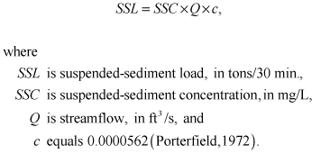 (1)
(1)
The 30-minute suspended-sediment load values were summed to estimate the daily load. For each water year (from October 1 to September 30), the daily suspended-sediment load values were then summed to provide annual loads for each station. In addition, suspended-sediment loads and yields were calculated for each major turbidity event period. Yields were calculated by dividing the suspended-sediment load by each subbasin drainage area. Suspended-sediment yields allowed for more direct comparison across subbasins by normalizing for drainage basin size.
Turbidity is an optical property defined as the measurement of light commonly scattered at 90 degrees to the incident light by suspended particles in an aqueous medium (Uhrich and Bragg, 2003). Suspended sand, silt, and clay or other organic material can decrease water clarity by increasing turbidity. Turbidity is measured according to a variety of methods, both as obtained in the laboratory or in direct instream installations. Each method uses different technology, yields different results, and has its own advantages. The USGS reduced the ambiguity in turbidity measurement by defining a suite of reporting units: the most common instruments measuring in Nephelometric Turbidity Units (NTU), Formazin Nephelometric Units (FNU), and Nephelometric Turbidity Ratio Units (NTRU) (Anderson, 2005). Most instream turbidimeters measure turbidity in FNU using an infrared or monochrome light source (780–900 nanometers), whereas most laboratory instruments measure turbidity in either NTU or NTRU using white or broadband light (400–680 nanometers). Equipment that measures in FNU or NTU has one detector and measures the scattered light roughly perpendicular to the incident light. Equipment that measures in NTRU uses a combination of detectors that measure light at 90 degrees (or other angles) and calculate a ratio between detectors. The USFS, City of Salem, and the U.S. Army Corps of Engineers primarily use instruments that measure in NTU, whereas the USGS field equipment measures in FNU and lab equipment in NTRU. Different turbidity units are cited throughout this report, with the unit used depending on which agency collected the data.
The most problematic turbidity issue for the water-treatment facility is high-turbidity events of long duration. These events result from prolonged rainfall eroding or mobilizing clay-rich sediment sources in the North Santiam River basin. The clays introduced to streams include very small, less-than-0.05-µm (micron) smectite, halloycite, and kaolinite (Bates and others, 1998; Hulse and others, 2002; Georg Grathoff, Portland State University, written commun, 2004). These particles can absorb water, expand, and remain suspended for extended periods as “persistent” turbidity. Persistently turbid conditions create problems because small particles pass through water-treatment filters, requiring expensive flocculating materials to aid settling. In addition, turbidity levels can remain elevated for days to weeks, adding to the delay and expense in providing a cost-effective water supply.
In order to measure persistent turbidity, more than 230 storm and high-flow samples were collected. Persistent turbidity was defined as having turbidity greater than 10 NTRU at a specified water depth after 8.5 hours. The 10 NTRU value was selected because it was a comparable value of turbidity at which potential alternative processing measures would be taken at the water-treatment facility. The 8.5 hours of settling was determined as the time 0.002‑mm (clay-sized) particles take to settle a known distance under controlled laboratory conditions. A suite of laboratory “turbidity-decay curves” were developed for each of the monitoring stations on the basis of all samples collected at its location. The initial turbidity value of each turbidity-decay curve (time = 0.01 hours) and the persistent turbidity (time = 8.5 hours) were used to develop regression models for each monitoring station (table 3).
Using the regression models and setting the persistent turbidity equal to 10 NTRU, a critical initial turbidity (the turbidity value that would produce a persistent turbidity of 10 NTRU after 8.5 hours of settling) was determined for each monitoring station. That value was converted to FNU by using another regression model. The final threshold turbidity values were as follows: French, 170 FNU; Breitenbush, 89 FNU; Blowout, 76 FNU; Little North, 69 FNU; and North Santiam, 64 FNU (fig. 6).
Clay-water volume was calculated for each major turbidity event by using the procedures developed by Uhrich and Bragg (2003). When the measured instream turbidity value reached the threshold value, as mentioned above, the volume of water flowing past the monitoring station while the turbidity exceeded the threshold value was calculated. The volumes of clay-water related to each of the major turbidity events, as well as the annual totals for each year, were calculated for all monitoring stations to quantify major sources of clay-water in the basin.
The eight major turbidity events in this report were selected because they were high-turbidity events (greater than 250 FNU) that had known origins. Six of the events were precipitation driven, whereas the remaining two were glacially or snowmelt driven. Seven of the major turbidity events occurred upstream of Detroit Lake, where monitors were deployed for the entire period of record. Most of the major turbidity events were evaluated as 3-day events; however, the two glacial outwash (snowmelt-driven) events were single-day events.

![]() U.S. Department of the Interior | U.S. Geological Survey
U.S. Department of the Interior | U.S. Geological Survey
Persistent URL: https://pubs.water.usgs.gov/sir20075178
Page Contact Information: Publications Team
Page Last Modified: Thursday, 01-Dec-2016 19:51:35 EST
