Scientific Investigations Report 2007–5186
U.S. GEOLOGICAL SURVEY
Scientific Investigations Report 2007–5186
Annual mean loads for TN, TP, and SS were estimated using the USGS computer program Load Estimator, or LOADEST (Runkel and others, 2004). LOADEST uses a seven-parameter linear regression model that incorporates flow, time, and seasonal terms to estimate loads of mass over specified time periods (for this study, annual loads). The calibration and estimation procedures within LOADEST are based on three statistical estimation methods. However, the Adjusted Maximum Likelihood Estimation (AMLE) was most often used since the method is more appropriate when the calibration data set (time series of streamflow and concentration data) contains censored data. Once the model was calibrated, continuous daily mean values of streamflow were used as the independent variable to produce the annual load results for the specified years of interest (for this study, WYs 1997, 2000, and 2001). Mean load estimates, along with standard errors, and 95 percent confidence intervals were computed. The LOADEST output also included diagnostic tests and warnings to assist the user in determining the appropriate estimation method and in interpreting the estimated loads. LOADEST is available as a USGS module (David Lorenz, USGS library for S-PLUS, version 6.1, for Windows—Release 2.1) to the S-PLUS statistical software package (Insightful Corporation, 2002).
The focus of the load computations for the specified years of interest was two-fold:
Results of the LOADEST modeling are in appendix A. Included in the appendix are annual loads, annual average flow-weighted concentrations (defined as the annual load divided by the cumulative annual streamflow), annual yields (defined as the annual load divided by catchment drainage area) for TN, TP, and SS, and annual mean streamflow.
The selection of the 11-year (WY 1993–2003) common time period for analysis of trends in streamflow, concentrations, and loads was based on a rigorous analysis of the temporal distribution of available USGS and non-USGS streamflow and water-quality datasets to optimize the number of sites spatially and temporally available for the analysis. An examination of annual mean streamflows for WY 1973–2003 in the Willamette Basin (fig. 3) illustrate how streamflows for WY 1993–2003 were representative of mean (average), high-flow, and low-flow years for the longer time period. This allowed the examination of water-quality trends and loads over a diverse and variable daily mean streamflow regime (Hirsch and others, 2006). The common time period occurred when the availability of ancillary data describing landscape, management practices, and climatic conditions were more accurately detailed. This ancillary information was important to the completion of the second and fourth study objectives. Attempts to extend the analysis period either forward or backward in time resulted in the loss of some sites considered important to the analysis. Comparison of streamflow during the selected 11-year period relative to the mean annual streamflow for WY 1973 (31 years of streamflow and water-quality data) also demonstrates the diverse nature of the common time period selected for the trend analysis (fig. 4).
Computation of annual mean loads of nutrients and SS in the Columbia and Puget Sound Basins was accomplished by selecting high, low, and mean streamflow years from the common period, WY 1993–2003. Six streamflow sites in Oregon, Idaho, and Washington were selected to characterize differences in climatic and hydrologic conditions in the eastern and western parts of each State within the basins (table 2). Although the peak daily streamflows generally occurred in WY 1996, the highest annual mean streamflows generally were during WY 1997, when streamflows ranked in the 93rd to 100th percentile of the highest annual streamflows in WYs 1973–2003. The lowest annual mean streamflows generally were during WY 2001, when streamflows ranked in the 1st to 14th percentile of the lowest annual streamflows in WYs 1973–2003. Selection of a mean annual water year representative of historical annual streamflow was more difficult because several water years in the common time period had annual streamflows similar to the historical mean annual streamflow. During the 1993–2003 period, WY 2000 best demonstrated monthly mean streamflows that were comparable to the means of the monthly streamflows from the historical time period (fig. 5). For these six index sites, the annual mean streamflows for WY 2000 ranked in the 48th to 76th percentile of the WY 1973–2003 mean annual streamflows.
Two types of data compilations were used in our analysis based on different minimum data requirements. The first type considered the selection of a consistent timeframe of daily mean streamflows and periodic sampling of water-quality constituents of a sufficient duration for the computation of trends in concentrations and loads of nutrients and SS. The minimum data requirements for the selection of sites for trends in concentration included:
These data requirements provided a minimum of 32 or more water-quality samples for each site used for the trends analysis (David K. Mueller, U.S. Geological Survey, written commun., 2005). Streamflow and water-quality data from 50 sites (table 1) met the minimum requirements for the analysis of trends in concentrations and loads.
The second type of data compilation considered the selection of streamflow and water-quality sites for computing annual loads and yields of nutrients and SS over a range of years. The 50 sites that met the minimum data requirements for the analysis of trends in concentration and loads also met the minimum load and yield selection requirement. However, these sites provided insufficient coverage of the Columbia River and of the Puget Sound Basins. An additional 50 sites were identified that met the less rigorous requirements for the second type of data compilation analysis. All sites for the second type of data compilation met the following minimum requirements:
One hundred sites met the minimum requirements for the second type of data analysis (fig. 1, table 1). The distribution of drainage areas for the 91 delineated catchments used in this study (delineations were not available for the other 9 sites) is shown in figure 6. The drainage areas ranged in size from 5 km2 to more than 650,000 km2; and, although the average drainage area was about 23,500 km2, most catchment drainage areas (54 of 91) were between 100 and 5,000 km2. All sites were reviewed for compliance with various modeling requirements (water-quality sampling representative of the flow regime for the period of interest, percentage of sampling results censored, confidence intervals, and other statistical measurements of model suitability).
Analyses evaluated for this study consisted of a suite of nitrogen, phosphorus, and SS data collected and analyzed by the USGS, other Federal and State agencies in Oregon, Washington, and Idaho, and a wastewater- and stormwater-treatment public utility in Oregon. To aid in the interpretation of the data, assumptions concerning varying sample collection protocols, equipment, and analytical techniques were made. A detailed discussion concerning the first two assumptions is presented in the next section.
The chemical and physical parameters used in this study included:
The above parameters were used to model loads, and trends in concentrations and loads, for TN, TP, and SS in the Columbia River and Puget Sound Basins for WYs 1993–2003. Where direct measurements of TN were not available, TN was computed from the sum of TKN and nitrite plus nitrate, using the rules outlined in table 3. The most common analytical reporting levels during WY1993–2003 were 0.2 mg/L for TKN and 0.05 mg/L for nitrite plus nitrate. In recent years, some slightly lower TKN and nitrite plus nitrate reporting levels were measured at some USGS and non-USGS sites; however, the rules were not changed significantly because it affected only a small number of the more pristine TN sites.
To produce a data set with adequate spatial and temporal coverage, it was necessary to include water-quality results from non-USGS as well as USGS data bases. As mentioned in the previous section, the validity of this approach partly rested on two assumptions: (1) differences between collection techniques using grab sampling (non-USGS) versus depth-width integrating sampling (USGS) were minor during typical flow regimes; and (2) differences in analytical techniques between various agency laboratories were minor. The WDOE compared their water-quality data to water-quality data collected during the same months by the USGS for two stations that also are included in this study (Hallock, 2005). The ranges for data collection were September 1982 through September 1994 for the Yakima River at Kiona, Wash. (Kiona), and December 1992 through September 2002 for the Palouse River at Hooper, Wash. (Hooper). USGS SS concentrations were significantly greater than the WDOE suspended-solids concentrations at Kiona on the basis of the central tendency of the data, but the difference in concentrations was not large and might have been due to differences in analytical techniques. In addition, concentrations were not significantly different between the two agencies’ data from the Hooper site. However, even a small bias at high concentrations and during high-flow periods for constituents positively correlated with flow (for example, SS and TP), caused fluxes to be magnified. SS and TP fluxes calculated from WDOE data were equal to 80 percent of the fluxes calculated from USGS data at Kiona and 50 percent of the USGS fluxes at Hooper.
Martin and others (1992) compared water-quality data collected concurrently using surface-grab and depth-width integrating sampling. Although concentrations of dissolved constituents were not consistently different, concentrations of SS and constituents associated with sediment were significantly lower in the surface-grab samples than in the depth-width integrated samples, and the magnitude of the differences generally increased with streamflow. Gray and others (2000) evaluated 3,235 paired samples of suspended-sediment (used by USGS) and total suspended-solids (used by the ODEQ and WDOE) and concluded that data resulting from the suspended-sediment techniques were more reliable, but that the methods may be comparable when the amount of sand-sized material is less than about 25 percent. Comparisons of concurrent nutrient samples (TN and TP) using standard USGS methods of analysis and methods of analysis used by non-USGS laboratories were not available.
For this study, comparisons also were made between model-predicted annual loads from a minimum of three co-located sites for the 3 water years of interest—high flow in 1997 (three sites), mean flow in 2000 (three sites), and low flow in 2001 (four sites). Table 4 summarizes the results of these comparisons by showing the predicted annual non-USGS load as a percentage of the predicted annual USGS load. The water-quality data used for the predictions were not collected concurrently, but all data were collected between WYs 1993 and 2003. For TN, the differences between the USGS and non-USGS loads generally were small (less than 10 percent) for all 3 years. However, for TP and SS, the non-USGS loads were less than the USGS load at all the sites in 1997 and 2000 (as low as 38 percent for TP and 31 percent for SS). As expected, SS was the most sensitive to sampling methodology and (or) laboratory procedures with regard to loads.
Results from other studies and the comparison of our co-located sites showed that surface-grab samples were biased low for elevated concentrations of sediment by as much as 70 percent and biased low for total phosphorous associated with high-flow conditions by as much as 60 percent. This deficiency might compromise load calculations if a stream is further stratified (fine particles and less mass near the top and heavy particles and more mass near the bottom). However, the results also showed that no persistent bias existed for total nitrogen (the differences were less than 8 percent). The value of using non-USGS load data to fill the spatial gaps in the USGS data outweighed the potential underestimation problems for TP and SS loads.
Changes over time in the concentration and load of a constituent can be used to evaluate the potential effects on water quality of changes in pollution sources or management activities in a watershed. However, the concentration and load of a constituent in a stream is influenced by the volumetric flow at the time of sampling (for example, higher concentrations and loads are generally associated with higher flows). This association is stronger for sediment and sediment-adsorbed constituents, like phosphorus, than for constituents that tend to dissolve in water, such as nitrate. However, an inverse relation may occur when a stream’s major source of nutrients is from point sources.
The relations of discharge to total nitrogen and discharge to suspended-sediment concentrations for Willamette River at Portland (fig. 1, site 33) for WY 1993–2003 are shown in figure 7. A locally weighted scatter plot smoothing (LOWESS) curve was fit to the data to indicate the relation between the parameters in the plots. Changes over time (trends) in the measured concentrations for a constituent (referred to as non-flow-adjusted trends in concentration) give an indication of water-quality changes streams have undergone. This is important with regard to possible effects on biota (for example, eutrophication). However, to determine whether a stream has experienced a trend in water quality due to changes in catchment activities, the effect of streamflow may need to be removed from the measured concentrations (because the streamflow itself might exhibit a trend). This is done by calculating the flow-adjusted trend in concentration, which gives insight into whether a trend in measured concentrations is potentially caused by management activities or reflects a trend in streamflow due to climatological or hydrological changes.
A detailed description of the method used in this study for estimating trends in streamflow, load, and concentration is provided in appendix B. Trends in load and concentration are defined as the model-estimated, smoothed trend in load and concentration over the period of water-quality record, divided by the length of record.
Smoothing of data is necessary when a measured variable is slowly varying and also influenced by random noise. In such a case, it is sometimes useful to replace each measured value with some kind of local average of the surrounding data points, thus reducing the level of variation without biasing the value of interest. An example of data smoothing (using a LOWESS curve) is shown in figure 8 which contains the measured daily mean streamflow and total nitrogen concentrations for the Willamette River at Portland for water years 1993–2003. Although LOWESS smoothing was used as an example in these plots, a different data smoothing routine was used for the analytical aspects of this study (see appendix B).
Because the water-quality record for most sites does not include enough data to assess trends in load and concentration, a mathematical model is needed to “fill in” the gaps in the water-quality record by estimating concentrations based on streamflow. The model-estimated trend in load and concentration is determined by fitting separate trend models for streamflow and water-quality concentration. The model for trend in streamflow relates the natural logarithm of daily mean streamflow to an intercept, a linear trend term (measured by time expressed as a decimal, such as 1995.5), and sine and cosine seasonal factors (also functions of decimal time). In this study, the trend was based on all daily streamflow measurements available over the analysis period WY 1993–2003 (except for the four sites where the record started in WY 1994). Below is a summary of the methods used to calculate non-flow-adjusted trend in concentration, trend in load, flow-adjusted trend in concentration, and trend in streamflow. Appendix B contains a formal description of the methods described below, with additional discussion of the estimation of the streamflow and water-quality models, and an explanation of the associated statistical tests for trend.
The water-quality model used to determine nonflow-adjusted trend in concentration (percent per year), estimated from all water-quality measurements collected during the analysis period, is represented by the following linear equation:
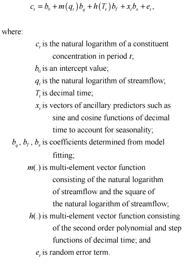 (1)
(1)
The smoothed trend in the natural logarithm of water-quality concentration (non-flow-adjusted trend in concentration) is determined by the streamflow and time trend components of the water-quality model (equation 1), where the smoothed trend in the natural logarithm of streamflow is substituted for the actual natural logarithm of streamflow in the model. The smoothed trend in the natural logarithm of streamflow is given by the following equation:
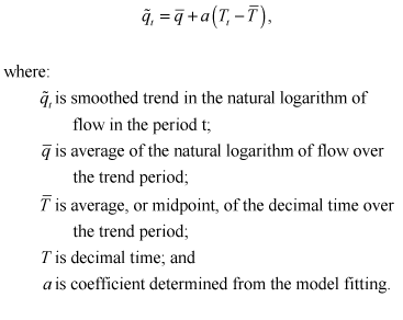 (2)
(2)
Non-flow-adjusted trend in concentration is obtained by transforming the model-estimated, smoothed water-quality trend from logarithmic space to real space, computing the percentage change corresponding to the first and last dates of the water-quality record period, and normalizing by the decimal time length of this period.
Trend in load (percent per year) is computed in a similar manner as non-flow-adjusted trend in concentration, except that the smoothed trend in the natural logarithm of streamflow is added to the smoothed trend in the natural logarithm of water quality prior to retransformation to real space (addition in logarithmic space is equivalent to multiplication in real space).
The estimation of flow-adjusted trend in concentration (percent per year) is similar to the approach used for non-flow-adjusted trend in concentration, except the streamflow component of the water-quality model is not included in the determination of the smoothed water-quality trend. Otherwise, the estimation methods are the same; that is, although flow is used to estimate the parameters of the water-quality model, implying that the trend parameters of the model exclude the effects of trend in flow, the flow component of the model is held constant and, therefore, does not enter into the evaluation of flow-adjusted trend.
The estimation of the trend in streamflow is based on the smoothed streamflow trend corresponding to the simple linear function of decimal time described by equation 2. The conversion of this smoothed trend to a trend estimate follows the same procedure described for non-flow-adjusted trend in adjusted concentration—the only difference is the period of the trend is taken to be the beginning and ending dates for the flow record within the analysis period, rather than the beginning and ending dates of the water-quality record.
Trend results also are reported as unit trends (for example, kilograms per day per year for load or milligrams per liter per year for concentration). The unit trends in load and concentration are determined by multiplying the load and concentration trend estimates (expressed as rates rather than percentages) by the appropriate reference values of load and concentration. The reference value for the natural logarithm of concentration is obtained by evaluating the water-quality model given by equation 1 at reference conditions consistent with the trend in water quality at the beginning of the water-quality period of record. These conditions include setting the natural logarithm of streamflow to the smoothed trend value given by equation 2 to the first day of the water-quality period, setting the trend term to the decimal equivalent of the first day of the water-quality period, and setting the sine and cosine seasonal factors to their average values over the full water-quality period. The natural logarithm value of the reference concentration is transformed to real space and a multiplicative retransformation factor is applied to correct for statistical bias arising from sample error in the water-quality model coefficients (see appendix B for additional details). The reference load is computed similarly, except that the natural logarithm of streamflow trend, as determined by the linear streamflow equation evaluated at the starting date of the water-quality period, is added to the natural logarithm value of the reference concentration prior to transformation to real space. In addition, a conversion factor is used to convert the result to the appropriate load units. The same reference concentration is used to derive non-flow-adjusted unit trend and flow-adjusted unit trend in concentration, and the same reference load is used in the evaluation of unit trend in load.
If streamflow demonstrates no trend over time, the non-flow-adjusted and flow-adjusted trends concentration will be equivalent. Because the water-quality model used to derive these trends includes streamflow as a predictor, the estimates of trend are immune to bias arising from preferential water-quality sampling during high-streamflow events. Care should be taken, however, in interpolating or extrapolating these trend estimates within or beyond a site’s period of record, or in making comparisons of trend across sites with different periods of record. Due to the possible nonlinearity of trend, as may arise from nonlinear specifications of the water-quality model streamflow or trend components, trends of shorter duration within the water-quality period of record, or trends occurring outside this period could be different from the trends reported here. In addition, the method used to evaluate trend is sensitive to changes in the variability of streamflow and to changes in the unexplained variability of water quality (both changes may potentially cause trends in water quality arising from nonlinearity in the specification of the water-quality model). Accommodation of these properties of the variance in the data effects awaits future research.
Annual TN and TP point-source loads were estimated for WY 2000 for the 91 delineated catchments (9 sites did not have delineated catchments). SS point-source loads were assumed to be negligible compared to in-stream SS loads and, therefore, were not estimated. Facility-specific average discharge, TN concentrations, and TP concentrations for WY 2000 were used to estimate the annual nutrient loads from each point source. Point sources without a measured discharge were assigned a discharge equal to the design flow rate. When WY 2000 nutrient concentrations were not available, facility-specific values for water years that were as close as possible to WY 2000 were used instead in an attempt to represent typical WY 2000 operations. When facility-specific nutrient concentrations were not available, region-wide average concentrations for the applicable standard industrial classification (SIC) category were used. When region-wide average nutrient concentrations for a SIC category were not available or the regional data set was not large enough, national typical concentrations for the applicable SIC code were used (obtained from the USEPA [Gerard McMahan, U.S. Geological Survey, written commun., 2006]). Loads were not calculated for facilities without a measured discharge, design discharge, or any available nutrient concentrations (site-specific, regional average, or typical national). In most cases, TN was not measured directly, so the components of TN (total Kjeldahl nitrogen [TKN] and dissolved nitrite plus nitrate as N) were summed to obtain a TN concentration. If the average WY 2000 value for a measured component of TN or TP was greater than the region-wide average for TN or TP, the facility-specific average value for the component was used (since the values for TN and TP cannot be less than their individual components). Water-quality and discharge monitoring reports were obtained directly from the facilities or from the USEPA Permit Compliance System (PCS) (U.S. Environmental Protection Agency, 2006a), a database containing State discharge monitoring reports (DMRs) (NPDES Discharge Monitoring Reports) submitted by the facilities.
All municipal wastewater-treatment plants (WWTPs) designated as major sources (design flow greater than 1.0 Mgal/d) were included in the analysis. The potential underestimation of loads caused by not including the minor WWTPs was determined by estimating the minor WWTPs contribution to the total annual discharge for all of the facilities in the Columbia Basin. If all the minor WWTPs were operating at 1.0 Mgal/d (an unlikely situation), they would comprise about 20 percent of the total annual WWTP discharge (and load). However, if all the minor WWTPs were operating at 0.5 Mgal/d (probably still a high estimate), they would comprise about 12 percent of the total annual WWTP discharge (and load). All non-WWTP facilities in the PCS falling under the SIC categories in table 5 were included in the analysis (regardless of size). The USEPA has determined that these SIC categories are large sources of industrial nutrient loads (Tetra Tech, Inc., 1998).
Locations of the 140 point sources with estimated TN loads and 130 point sources with estimated TP loads in the catchments included in this study for WY 2000 are shown in figure 9. Point sources discharging directly to the Puget Sound are not shown in figure 9, but are discussed in the section describing that system. The sources are color-coded and sized to represent their relative loads based on the quartiles for annual TN and TP loads. Table 6 shows the ranges for the annual WY 2000 point-source load quartiles. The point sources with the largest nutrient loads were located around major population centers (lower Columbia River Basin, Willamette River Basin, Snake River Plain, near Spokane, Yakima River Basin, and the confluence of the Yakima, Snake, and Columbia Rivers).

![]() U.S. Department of the Interior | U.S. Geological Survey
U.S. Department of the Interior | U.S. Geological Survey
URL: https://pubs.usgs.gov/sir/2007/5186
Page Contact Information: Publications Team
Page Last Modified: Thursday, 01-Dec-2016 19:52:39 EST
