Scientific Investigations Report 2007–5237
U.S. GEOLOGICAL SURVEY
Scientific Investigations Report 2007–5237
Computer models were used to simulate the physical and chemical processes affecting the fate of nitrate in the shallow aquifer system near La Pine. The purpose of developing the models was to (1) test concepts of how hydrogeologic and geochemical processes affect the movement of nitrate through the ground-water system, and (2) provide tools that could be used to evaluate future water-quality conditions and alternative management options. This section describes the process of constructing and calibrating simulation models at two scales: (1) a transect model used to estimate model parameters and boundary conditions along a ground-water flow path where there is a detailed understanding of the flow system and geochemical evolution of ground-water, and (2) a study-area model covering the area where there are water-quality management concerns.
This section includes: (1) discussion of the overall modeling approach used to construct and calibrate the transect and study-area models, (2) discussion of model parameters that must be specified for both models and how the values were estimated and modified during calibration, (3) discussion of hydrologic stresses specified for both models, (4) a detailed description of boundaries, discretization, and calibration of the transect model, and (5) a detailed description of boundaries, discretization, and calibration of the study-area model. Alternative management options were evaluated first by using the study-area model to simulate prescribed scenarios and then by coupling the study-area model with optimization methods. The coupled simulation and optimization model is referred to as the Nitrate Loading Management Model (NLMM).
The study-area model includes 247 mi2 of southern Deschutes and northern Klamath Counties (fig. 10) where either existing or planned future development uses on-site wastewater systems. The study-area model was used to simulate the long-term effects of historical and future nitrate loading from on-site wastewater systems on ground-water quality in the study area.
The transect model is more detailed and includes 2.4 mi2 of the shallow aquifer system near Burgess Road (fig. 10). The transect model was used during the calibration process to (1) test basic concepts of ground-water flow and nitrate fate and transport, and (2) refine estimates of model parameters through calibration in part of the study area where abundant geologic, hydrologic, and chemical data were available to constrain the model.
A regional ground-water flow model of the 4,500 mi2 upper Deschutes River basin was developed by Gannet and Lite, (2004) to address issues of water supply and ground-water/surface-water interaction. The model does not have the capability to simulate transport of nitrogen and the resolution (grid cell size) of the model grid is not adequate near La Pine to make this model an effective tool for addressing issues related to on-site wastewater systems. The regional model was used, however, to specify initial values of parameters and boundary conditions for the study area and transect models.
The first step in developing the transect and study-area models was to construct a ground-water flow model and simulate the velocity and direction of ground-water movement. This velocity distribution then was used in a solute-transport model to simulate the advection and dispersion of nitrate in the ground-water system. Steady-state flow conditions were assumed for the ground-water velocity distribution; that is, it was assumed that there were no changes in storage and the direction of ground-water flow and velocity did not significantly change during the simulation period. The steady-state flow models (transect and study area) were calibrated using observations (measurements) of hydraulic head, ground-water discharge rates to rivers, and chlorofluorocarbon (CFC) based time-of-travel estimates (Hinkle and others, 2007a). The accuracy of the transport model was evaluated by simulating nitrate loading during the 40-year period 1960–99 and comparing statistical distributions of observed and simulated ground-water nitrate concentrations.
Ground-water flow and nitrate transport were simulated using the programs MODFLOW-96 and MT3DMS. The U.S. Geological Survey’s MODFLOW model (Harbaugh and McDonald, 1996) is a numerical simulation program capable of simulating hydraulic heads and ground-water flow within a three-dimensional system. The MT3DMS simulation program (Zheng and Wang, 1999) uses the velocity field computed by MODFLOW to simulate the movement of dissolved chemical species in ground water due to advection and dispersion. MT3DMS also is capable of simulating the effects of chemical reactions on the concentration of dissolved species.
The study-area and transect models developed for this study consist of a set of data input files that specify the boundary and initial conditions, the hydraulic and transport parameters, and the hydraulic and chemical sources and sinks specific to the study area. These input files provide the data required by the model programs (MODFLOW-96 and MT3DMS) to solve a complex set of partial differential equations that compute ground-water head and flux as well as solute concentration and flux in the subsurface.
Several parameters must be specified for each cell in a model. These parameters, hydraulic conductivity, porosity, and dispersion coefficient, define the characteristics of the porous medium (geologic materials) that control the movement of ground water and the fate and transport of nitrate.
Initial values of hydraulic conductivity for the five major lithofacies in the hydrogeologic model were estimated using (1) results from 24 slug tests done for this study, (2) analysis of 221 well-yield tests reported by drillers, and (3) literature values. The three fluvial hydrofacies, clay-silt, sand, and gravel, were assigned values of 3, 25, and 57 ft/d, respectively, based on mean values from the slug tests. The lacustrine clay-silt hydrofacies was assigned a value of 1 ft/d. The initial value for the basalt hydrofacies was 800 ft/d based on values used by Gannett and Lite (2004) in the La Pine study area. The initial values of vertical hydraulic conductivity were derived by adopting the horizontal to vertical anisotropy ratio of 1,000 used in the regional model for the La Pine study area (Gannett and Lite, 2004). The resulting initial values of vertical hydraulic conductivity were 0.001, 0.003, 0.025, 0.057, and 0.8 ft/d for the lacustrine clay-silt, fluvial clay-silt, fluvial sand, fluvial gravel, and basalt hydrofacies, respectively. Initial values of horizontal and vertical hydraulic conductivity were assigned to each cell in the model on the basis of the hydrofacies represented in the cell.
Effective porosity is defined as the amount of interconnected pore space and fracture openings available for the transmission of fluids, expressed as the ratio of the volume of interconnected pores and openings to the volume of rock (Lohman, 1972). Effective porosity generally is smaller than the total porosity of the porous medium, reflecting that some pore spaces may contain immobile water with zero ground-water seepage velocity (Zheng and Wang, 1999). However, as discussed in some detail by Zheng and Bennett (1995), this so-called effective porosity cannot be readily measured in the field due to the complexity of the pore structure. Rather, it generally must be interpreted as a lumped parameter and estimated during calibration by comparison of simulated and observed solute movement or ground-water travel time. An initial value of 0.30 was used for the effective porosity of all five hydrofacies.
The solute transport model includes the process of dispersion to account for factors such as diffusion, flow path tortuosity, and heterogeneities in the porous media that cause velocities to deviate from the average seepage velocity. The geostatistical method used to simulate the distribution of hydrofacies allowed the model to represent a great deal of the large scale heterogeneity in hydraulic properties. The scale of heterogeneities incorporated in the hydrogeologic model was, however, limited to the scale of the model grid (200 and 500 ft laterally for the transect and study-area models, respectively, and 5 ft vertically for both models). Because much of the heterogeneity occurs at scales that cannot be represented by a grid cell, the dispersion coefficient was used to represent the smaller (sub-grid cell) scale heterogeneity of the system. Additional factors, such as temporal variations in recharge rates and flow directions that affect solute transport often are incorporated into simulations as dispersion (Goode and Konikow, 1990).
Dispersion is represented by three dispersivity coefficients—one for longitudinal dispersivity, which represents dispersion along the primary flow axis, and two for transverse dispersivity values, which represent dispersion in the horizontal and vertical directions normal to the axis of flow. MT3DMS allows the user to specify the longitudinal dispersivity for each model layer and to set the transverse horizontal and transverse vertical dispersivity values as a fraction of the longitudinal dispersivity. The initial value for the longitudinal dispersivity was set to 50 ft to represent sub-grid cell heterogeneity. Typically, the horizontal transverse dispersivity is much smaller than the longitudinal dispersivity and the vertical transverse dispersivity is smaller still (Zheng and Bennett, 1995). Initial values for the transverse dispersivity were set to 5 and 0.5 ft for horizontal and vertical, respectively. The final, calibrated longitudinal, transverse, and vertical dispersivity values were 60, 6, and 0.06 ft, respectively.
Model stresses are the flows in and out of the ground-water system that are specified or simulated by the model. The stresses include recharge, discharge to springs and by evapotranspiration (ET), and exchange between streams and the ground-water system. Discharge by pumping wells is another stress, however it was not included in the model because seventy-five percent of domestic well pumping is returned as recharge from on-site wastewater systems. Recharge is the only specified stress in the models; other stresses are simulated by the model based on relations between head in the ground-water system and stream or springs elevation or the rooting depth of plants that discharge ground water by ET.
Specified flux and head-dependent flux boundary conditions were used to simulate movement of water between the ground-water system and streams, springs, and the atmosphere. Recharge by infiltration of precipitation was represented by specifying flux to the water table using the recharge (RCH) package (Harbaugh and McDonald, 1996). Streams and rivers, springs, and evapotranspiration were represented using head-dependent flow boundary options in MODFLOW-96 (RIV, DRN, and EVT packages). The locations of cells designated as head-dependent flux boundaries are shown in figure 10.
The distribution of recharge by infiltration of precipitation and snowmelt was estimated for the upper Deschutes basin by Gannett and others (2001) using the Deep Percolation Model (DPM) of Bauer and Vaccaro (1987). The basin was modeled using a grid with cell dimensions of 6,000 ft per side. Gannett and Lite (2004) used estimated 1993–95 mean annual recharge to simulate steady-state conditions. The 1993–95 recharge distribution was used as the initial estimate of recharge to the study-area model; values for each cell were derived by overlaying the study-area model grid with the DPM model grid using a GIS (fig. 5). Neither recharge from on-site systems nor withdrawals by domestic wells were included in the model because, in the context of the overall water budget, these components are essentially equal and offsetting. Reductions in water level near pumping wells are not represented in the study-area model using this approach. Individual domestic wells may influence ground-water flow within localized areas (a few cells), but they would not have a significant effect on the direction and rate of ground-water flow at the scale the model is intended to be used.
Ground-water discharge to and recharge from streams was simulated with the river (RIV) package of MODFLOW-96 (Harbaugh and McDonald, 1996). Data required by the RIV package include: mean stream stage, stream-channel elevation, and streambed conductance for each cell that contains a stream. All major streams in the study area were simulated using this method (fig. 10).
All stream-channel elevations were estimated using a 10-m digital elevation model (DEM). The mean stage was estimated to be 4 ft above the streambed in the Deschutes River, 2 ft above the streambed in Paulina Creek and Little Deschutes River, and 1 ft above the streambed in Long Creek. Streambed conductance (SC) is calculated using the equation:
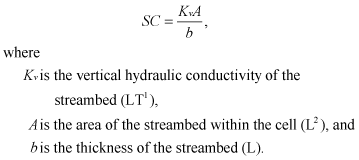
Conductance values were variable depending on the hydrofacies of the cell and the area of the stream within the cell. The initial conductance values were calculated by assuming that the vertical hydraulic conductivity of streambed sediments was 1/100th of the horizontal hydraulic conductivity of the cell. Streambed thickness was set to 1 ft throughout the model.
Ground-water discharge to springs was simulated with the drain (DRN) package of MODFLOW-96 (Harbaugh and McDonald, 1996). Data required by the DRN package include the spring elevation and conductance for each cell that contains a spring. This package was used to represent discharge from springs at the contact between the basin-fill sediments and volcanic rocks on the west side of the Deschutes River between the confluence with Spring River and the northern boundary of the model (fig. 10). All spring elevations were estimated using a 10-m digital elevation model (DEM) data. The conductance parameter has the same dimensions (L2T-1) as the streambed conductance; however, the parameter cannot be easily related to measurable physical characteristics of the springs. Initial values of conductance ranged from 5,000 to 10,000 ft2/d and were adjusted during calibration.
Discharge from the water table by evapotranspiration (ET) was simulated using the EVT package of MODFLOW-96 (Harbaugh and McDonald, 1996). ET can occur where plants with roots extending to the water table (phreatophytes) use ground water for transpiration or where the water table is close enough to land surface to allow direct evaporation from bare soil. The EVT package uses the assumption of a linear relation between ET discharge and depth to the water table. Data required to define this relation are the potential ET rate (LT-1), depth below land surface at which ET ceases (extinction depth), and land surface elevation (L). The potential ET rate was specified as 1.0 ft/d, the extinction depth was 5 ft, and the land surface elevation was specified from DEM data. Only cells where the water table was estimated to be within 10 ft of land surface were activated in the EVT package (fig. 10). The nitrate concentration in ground water used by plants in the ET process was specified as zero because the (1) part of model-simulated ET that is due to plant transpiration (as opposed to evaporation from bare soil) could not be determined, and (2) nutrient uptake by phreatophytes is species dependent and not well constrained.
The transect model was developed for a part of the ground-water system near Burgess Road (fig. 10). This area was selected for detailed scale modeling because it was the site of intensive data collection and study of changes in ground-water age and chemistry along a ground-water flow path transect (Hinkle and others, 2007a). The 3.5-mi long transect model comprises 17 wells at 6 sites (2–4 wells per site) aligned with the predominant direction of ground-water flow (fig. 11). In addition to ground-water age and chemistry data, hydraulic head, lithologic data, and hydraulic conductivity data were available from the transect wells to construct and calibrate the transect model.
The boundaries of the transect model (fig. 11) were selected to coincide with hydrogeologic boundaries of the local flow system. The western boundary of the model is a no-flow boundary defined by the ground-water divide that coincides with the surface-water drainage divide between the Deschutes and Little Deschutes Rivers. The north and south boundaries of the model are streamline boundaries that parallel the principal direction of ground-water flow from the drainage divide to the Little Deschutes River. The Little Deschutes River, a discharge area, was simulated as a head-dependent flux boundary. The initial conceptual model of the system included a deep regional component of upward ground-water flow across the lower model boundary. The concept for the lower boundary was evaluated by applying a specified flux across the lower model boundary based on data from the regional ground-water flow model by Gannett and Lite (2004). The upward flux estimates from the regional model did not allow a good simulated match to observed conditions (head and flux) when hydraulic conductivity and recharge values were within reasonable ranges based on independent data. Little or no upward flow from a deep regional source is needed to simulate the observed distribution of head and estimated ground-water flux to the Little Deschutes River. Upward vertical gradients were measured in well pairs in the area and geochemical evidence indicates that ground-water discharge to areas near the rivers may have a deep regional component (Hinkle and others, 2007a). Seepage estimates and simulations using the transect model, however, indicate that the magnitude of regional discharge must be small compared to local recharge to the shallow alluvial aquifer. The lower boundary of the transect model was specified as a no-flow boundary.
The numerical methods used by MODFLOW and MT3DMS to solve the equations for ground-water flow and solute transport require that the ground-water system be divided into discrete rectangular volumes, called cells. The rows, columns, and layers of cells that make up the three-dimensional array are collectively referred to as the model grid. The center of each cell defines a point at which the hydraulic head and solute concentration is simulated. The simulated head and concentration values are taken to represent the average values within the cell.
The longest dimension of the model grid was aligned to the principal direction of ground-water flow from west to east. The grid consists of 18 rows, 92 columns and 15 layers of cells, with each cell having dimensions of 200 ft in the row and column directions and 5 ft in the vertical direction. The three-dimensional transect model was 3.5 mi in the east-west (column) direction, 0.7 mi wide in the north-south (row) direction (normal to the principal direction of flow), and 75 ft thick in the vertical (layer) direction (fig. 11).
A three-dimensional hydrofacies model of the fluvial and lacustrine sediments within the transect flow model was constructed using the methods previously described for constructing the hydrofacies model for the study-area model. A sectional view through the model along row 8 is shown in figure 11C and illustrates the heterogeneity of the fluvial sediments. Transition probability geostatistical methods were used with the same model parameters (mean lengths, transition probabilities, and proportions) as were used for the study-area hydrofacies model, however the transect hydrofacies model was discretized into cells with the same dimensions as the transect simulation model.
The MODFLOW model was first calibrated to steady-state flow conditions using head data from the June 2000 synoptic well measurement. Data were available from 26 wells within the transect model area (fig. 11); 17 wells were piezometers installed as part of the Burgess Road transect study and 9 were existing domestic water-supply wells.
Observations (either measurements or estimates) of ground-water discharge to streams were available to constrain model calibration; however, flux between the Little Deschutes River and the shallow ground-water system was difficult to characterize because of uncertainty in the seepage measurements. The apparent gains and losses for the 13-mi reach downstream of the gaging station (14063000) ranged from a 2.6 ft3/s gain in October 1995 to a 1.6 ft3/s loss in October 2000 (table 4). These 1995 and 2000 estimates were less than the estimated error of measurement (± 3.9 ft3/s and ±6 ft3/s, respectively). A third seepage measurement in March 2000 indicated a 12 ft3/s loss in this reach, but this loss was based on measurements at relatively high flow conditions (about 300 ft3/s) with a larger associated error. For calibration purposes, October low-flow data were interpreted to indicate that net seepage to or from this reach (1) is small relative to flow, and (2) probably varies in direction as well as magnitude depending on annual or seasonal head relations between shallow ground water and the stream. A key component of the conceptual model of the shallow flow system is that, on annual or longer time scales, there is net discharge to the Little Deschutes River. On this basis, a range of discharge to the stream for the transect model area was computed using the October 1995 seepage (2.6 ft3/s) as the minimum and the sum of seepage and estimated error of measurement (6.5 ft3/s) as the probable maximum for the range. Dividing seepage and estimated error of measurement by the length of the reach (13 mi) yielded a range of 0.20 to 0.50 ft3/s/mi and the resulting range of expected mean annual ground-water discharge to the 1.3 mi reach of the Little Deschutes in the model area was 0.3 to 0.7 ft3/s (rounded).
During the calibration process, parameters such as horizontal and vertical hydraulic conductivity, recharge, and streambed conductance were adjusted, using a trial-and-error procedure, to obtain the best fit between observed and simulated head and stream flux values. The transect model also was used to evaluate estimates of upward vertical flux across the lower boundary from the regional flow model.
Horizontal hydraulic conductivity (Kh) and vertical hydraulic conductivity (Kv) values were assigned to each cell according to the hydrofacies represented in the cell. The probable range of Kh based on well-yield data and slug tests and the calibrated Kh value that yielded the best model fit are listed in table 5. The probable range of vertical hydraulic conductivity for each hydrofacies was computed assuming that the probable range of the horizontal to vertical anisotropy ratio was 10 to 10,000 for the hydrofacies in the model area. The vertical anisotrophy ratio in the final model was equal to 100 for all hydrofacies.
Streambed conductance was estimated on the basis of the assumption that the vertical hydraulic conductivity in streambed sediments was 1/100th of the horizontal conductivity of the hydrofacies in the model cell. A series of simulations were made to test model sensitivity to streambed conductance values. Conductance values were modified by adjusting the ratio of streambed Kv to aquifer Kh, over a range of 0.001 to 0.1, but the transect model was relatively insensitive to this parameter.
Recharge estimates for the transect model area range from 1.5 to 2.1 in/yr. The lower end of the range was estimated by using a water balance model for the upper Deschutes Basin (Gannett and others, 2001); the upper end of the range was computed by using CFC-derived age data from the Burgess Road transect study (Hinkle and others, 2007a). The best model fit was obtained with a slightly higher recharge rate of 2.3 in/yr.
Hydraulic heads and discharge to the stream simulated by the transect model were most sensitive to recharge and horizontal hydraulic conductivity of the fluvial clay-silt and lacustrine clay-silt hydrofacies. The fluvial sediments are relatively thinner than the lower permeability lacustrine sediments near the river and this tends to reduce the composite transmissivity of the aquifer system. The location, thickness, and extent of clay-silt hydrofacies within the fluvial sediments are relatively unimportant factors controlling ground-water flow because the contrast in hydraulic conductivity between the gravel, sand, and clay-silt hydrofacies is small compared to the contrast between the fluvial and lacustrine hydrofacies. Fitting simulated to observed heads was accomplished by adjusting values of hydraulic conductivity for each hydrofacies, until a best model fit was obtained by trial and error.
The calibrated parameter values (table 5) and boundary conditions produced a good model fit to head and flux observations. Contours of simulated water-table elevation compare well with observed water-table elevations at 15 wells (fig. 11A) where measured heads represent the water table. The root mean square error (RMSE) of the head residuals at the 26 well locations was 2.7 ft. Model fit was slightly better (RMSE = 2.3 ft) at the 17 transect wells, where head measurements were more accurate because (1) measuring point elevations at the wells were surveyed, whereas elevations at other wells were estimated from topographic maps, and (2) short (2-ft) screens in the transect wells provided better observations of head within the 5-ft thick model cells, whereas screens in other wells were longer and spanned multiple model layers. The simulated heads have a slight bias that results in a steeper slope of the water table toward the Little Deschutes River. The bias probably could be reduced with further calibration if the configuration of the lacustrine-fluvial sediment boundary were modified; however, there was no basis (using existing geologic data) to modify the hydrofacies model and the bias was small and did not significantly affect average simulated flow velocities.
Estimates of ground-water age were used to further constrain the calibration of the transect model. Ground-water age estimates at 17 wells in 6 locations along the Burgess Road transect (fig. 11B, C) were derived from analysis of CFCs (Hinkle and others, 2007a). A particle tracking program, MODPATH, (Pollock, 1994) was used to determine the simulated travel time of ground-water from recharge locations at the water table to the well screens where CFC samples were collected from the 17 transect wells. The simulated travel times were compared with the CFC-derived age estimates to evaluate the accuracy of the simulated ground-water velocity distribution.
MODPATH uses the cell-to-cell fluxes simulated by MODFLOW to compute velocity field and path lines of individual “particles” of water that may be started at any location and tracked either forward to their discharge location or backward to their recharge location. The only additional parameter required by MODPATH (that is not required by MODFLOW) is effective porosity. Effective porosity was assumed to be 0.3 for each hydrofacies within the model. For this analysis, 1,000 particles were placed in each of the 17 model cells that contained the screen of a transect well. The particles were tracked backward to their recharge locations at the water table (fig. 11C). Because of limitations of the tracking program, particles could not be placed at the exact location of the well screens within each cell, but were placed at the center of the cell and distributed along a vertical line 5-ft long (the thickness of the cell).
Simulated ground-water travel time distribution is shown in figure 11B for row 8 of the transect model. The simulated distribution shows a pattern similar to the distribution of CFC-derived ages from the 17 transect wells. Generally, ground-water travel times are less than 10 years within the upper 5–15 ft of the saturated zone and travel times within 30–50 ft of the water table are less than 50 years. Simulated ground-water travel times are notably greater than CFC ages at well 4.3, the deepest at site 4. Travel times are difficult to predict at this site because the screen for well 4.3 is near the upper surface of the fine-grained, lacustrine clay-silt hydrofacies. The model predicts that “older” water will occur at this location because slow-moving water from the lacustrine sediments re-enters the fluvial sediments as it follows flow paths toward the discharge areas along the river. At the discharge end of the flow path, near the Little Deschutes River, older water occurs at shallower depths as it moves upward to discharge to the river. The relation between ground-water age and depth depicted in the section (fig. 11B) is analogous to the relation between dissolved oxygen concentration and depth described by Hinkle and others (2007a).
Initial estimates for many parameters in the study-area model were derived from calibration and testing of the transect model. The study-area model was first calibrated for simulation of ground-water flow using observations of head and discharge to streams. As with the transect model calibration, simulated heads were compared with water-level data from the synoptic measurement of 228 wells in June 2000 (fig. 5). Simulated ground-water discharge to streams was compared with estimates of discharge from gain-loss measurements (fig. 7, table 4). The measured head and discharge data were assumed to represent the long-term average (steady-state) conditions in the ground-water system. Once the study-area flow model was calibrated, the simulated ground-water flow directions and velocity were used to simulate the transport and fate of nitrate. Transport of nitrate from on-site wastewater systems was simulated for 1960–99 using the estimated annual nitrate loading rates. The transport model was evaluated by comparing the statistical distribution of simulated nitrate concentration with statistical distributions of measured nitrate concentrations from analyses available mostly from domestic wells.
The transport model calibration period was divided into 40 1-year stress periods. During each 1-year period, the nitrate loading rate in each model cell was specified. The specified rate was dependent on the number and type (domestic, commercial, etc.) of on-site wastewater systems present.
The model grid for the La Pine study-area model includes an area of 247 mi2 (fig. 10). The grid is elongated along a northeast-southwest trend that coincides with the orientation of the structural basin, major drainages, and the depositional strike and dip of the basin-fill sediments. The axes of the grid also are orthogonal to the principal directions of ground-water flow. There are 276 rows, 100 columns, and 24 layers in the model grid. The lateral dimensions of each cell are 500 ft in both the x and y directions. The upper 23 layers of the model were each 5 ft thick and the bottom layer was 100 ft thick. The coordinates of the lower left corner of the grid are 4,609,651 ft east and 696,295 ft north (Oregon State Plane north) and the grid is rotated 15 degrees clockwise.
The fluvial sand and gravel aquifers that supply most drinking water to wells in the area lie within the upper 100 ft of sediments. Between depths of 10 to 100 ft, depending on location in the study area, there is a transition from the coarser fluvial sediments to predominately fine-grained lacustrine sediments (fig. 2, pl. 1). As previously described, the fluvial deposits are heterogeneous and include fine-grained facies of clay, silt, and silty-sand. Similarly, coarse facies occur within the lacustrine deposits, although they tend to be isolated lenses. The simulation model was constructed to include the upper 120 ft of sediments so that the model would include the entire thickness of fluvial sediments. Each of the 24 model layers had a thickness of 5 ft throughout the grid. The grid for the study-area flow and transport model was defined to exactly match the dimensions of the grid used to prepare the three-dimensional hydrogeologic model described earlier in this report.
Long-term well hydrographs (fig. 6) indicate that ground-water flow in the shallow part of the system is in a state of dynamic equilibrium. Seasonal and interannual variations in water level and ground-water storage are due to climatic variation, but no long term trend is evident in mean water levels. The June 2000 synoptic water level measurements (fig. 5) were assumed to represent the mean annual head distribution for the system and were used as the head observations used as calibration targets for the steady-state study-area and transect flow models.
The lateral and bottom boundaries of the model were selected to include the most densely developed part of the study area and the shallow alluvial deposits that form the primary aquifers. The lateral and bottom boundaries of the model do not coincide with specific hydrologic or geologic boundaries such as geologic contacts or ground-water flow divides. The potential magnitude of flow across the lateral and lower model boundaries was evaluated by model testing and sensitivity analysis with both the transect and study area models. The upper boundary of the model is the water table, which is the top of the saturated part of the ground-water flow system.
The study area transport model used steady-state flow velocities to simulate nitrate fate and transport. Nitrate loading from on-site wastewater systems was simulated for 1960–99 in forty 1-year periods. The loading for each period was computed using building records and other information as previously described (fig. 9). Nitrate loading was specified in the transport model using the mass-loading option in the source/sink mixing package of MT3DMS (Zheng and Wang, 1999). The mass loading rate to each cell, in kilograms per day, was specified at the water table for each year of the simulation. Initial nitrate concentrations were assumed to be zero at the beginning of the simulation in 1960.
Based on the conceptual model for denitrification (Hinkle and others, 2007a), the transition zone from oxic to suboxic conditions was represented as a sharp boundary that does not vary significantly with time. Although the redox boundary would be expected to migrate as solid-phase electron donors are consumed by dissolved oxygen and nitrate reduction, the effectiveness of this approach for characterizing current zones of nitrate stability and instability is supported by analysis of data collected by ODEQ (Hinkle and others, 2007a). Hinkle presents field data from the area showing that 95 percent of samples with nitrate concentrations greater than 1.0 mg N/L taken from wells with known construction were screened at least partly within the mapped (fig. 8) oxic zone.
The position of the boundary within the models was specified by subtracting the thickness of the oxic part of the aquifer (fig. 8) from the water-table elevation (fig. 5) to obtain the elevation of the oxic-suboxic boundary. The boundary was assumed to be in each vertical stack of cells at the top of the first fully suboxic cell. The boundary was implemented in MT3DMS by using the ICBUND array to specify a constant concentration of zero in suboxic cells (Zheng and Wang, 1999).
Ground-water fluxes across the lateral and lower boundaries of the study-area model initially were specified on the basis of the regional ground-water flow model developed by Gannett and Lite (2004). The uppermost layer of the regional model was 100 ft thick and represented both alluvial deposits and basalts. The regional model simulates large subsurface flow through the permeable basalts that underlie the northern part of the study area (fig. 2). Most of the flow remains within the basalts of the regional flow system and discharges to the Deschutes River and tributaries north of the study area (Gannett and others, 2001). Some of the flow through the basalts, however, discharges to springs that contribute to the Deschutes, Fall, and Spring Rivers in the northwestern part of the study-area model. These springs generally are located where high permeability basalts abut lower permeability sediments, forcing ground water to discharge at land surface (Gannett and others, 2001).
Where alluvial deposits occur at the lower and lateral boundaries of the study area model, the flux simulated between the regional and study-area models was generally small. This is consistent with results of testing the transect model that indicated upward leakage across the lower boundary was not required to match the observed head distribution and ground-water discharge to streams when using reasonable values for recharge and hydraulic conductivity. This result indicates that upward leakage is small compared to local recharge from infiltration of precipitation.
When the simulated flux across the lower and lateral model boundary was included in the simulation, the study-area model had numerical stability problems in the northern part of the model area, which is underlain by basalt. The stability problems were characterized by large fluctuations in simulated heads that were probably caused by (1) a large flux through a relatively thin section (120 ft) of the basalts, and (2) adjacent model cells with large contrasts in hydraulic conductivity (high hydraulic conductivity basalts in immediate contact with low conductivity alluvial deposits).
To test the sensitivity of model results to specified flux at the lateral and lower model boundaries, a simulation was made specifying zero flux at these boundaries. Simulated heads and flux to streams were determined to be insensitive to the regional model boundary flux where basalts were not present. Few data points were available to constrain the heads in the basalt uplands and, therefore, even though simulated heads were affected in the basalts, it is difficult to assess how well or poorly they match actual heads. The simulated discharge to springs along the Fall, Spring, and Deschutes Rivers in the northern part of the model area also were affected, but the model showed much better stability. Nearly all potential concerns related to nitrate from on-site wastewater systems are focused on parts of the study area underlain by alluvial deposits. Simulation of flux through the basalts and of discharge from large springs at the basalt-alluvium contact was of less importance and did not inhibit the ability of the model to simulate conditions in the alluvial deposits; therefore, to attain better model stability in the part of the model representing basalts, the zero-flux boundary condition was used for the lower and lateral boundaries of the study-area model.
The contours defining the simulated steady-state potentiometric head surface retain the general features of the surface defined by contours of measured heads from the 2000 synoptic measurement (fig. 12). Both simulated and observed flow directions (inferred from contours) support other data (vertical head gradient and gain-loss measurements) that indicate, on an annual basis, ground water discharges to nearly all stream reaches in the study area.
The model simulated the general direction of ground-water flow (northeast) accurately in the area between the Deschutes and Little Deschutes Rivers in southeast T20S/ R10E and northeast T21S/R10E; however, the model did not simulate as steep a horizontal hydraulic gradient as indicated by the contours of observed heads shown in figure 12. The location of this area between the two rivers and at the focal point of ground-water flow for a large part of the study area, make it difficult to characterize the mean annual head distribution. Seasonal differences in the stage of the Deschutes and Little Deschutes Rivers can cause relatively large seasonal variations (5–10 ft) in ground-water levels. The period of high river stage in spring coincides with the peak recharge period for the shallow aquifer. These conditions lead to larger horizontal head gradients, particularly in this area, when the water levels used to construct the contours in figure 12 were measured (June 2000). The simulated recharge and river stage conditions represent mean annual conditions, as do the simulated heads, whereas the contours shown in figure 12 may represent a seasonal extreme. The transient influence of the rivers makes it difficult to accurately simulate ground-water flow velocity and direction in this area; however, the model simulates the mean annual direction of flow and velocity reasonably well. On-site wastewater systems are not used in this area so it is not likely that the model would be used to predict concentration in this area. Long Creek was represented in the model using head-dependent flux boundaries for ET and streams to account for discharge in the topographically low area; the effects of ground-water discharge are reflected in the V-shaped simulated and observed contours (fig. 12).
The mean absolute error for the 170 head observations was 7.0 ft, or about 5 percent of the range of observed heads. The difference between simulated and observed head ranged from -20 to 45 ft (fig. 13). The largest differences generally were at wells with long open intervals, in which the measured head represents a composite head for a large thickness of the system. The simulated heads used for comparison in such cases were for the model layer closest to the center of the open interval of the well. The differences between simulated and observed head generally were less than 10 ft in the central part of the study area, between the Deschutes and Little Deschutes Rivers. Errors in the simulated heads will result in errors in the ground-water velocity field that in turn will affect simulation of nitrate transport. These errors would affect simulated concentrations at small scales, but would not affect the average simulated nitrate concentration over large areas.
Recharge to the water table, which was 98 percent of total recharge, was the only specified component of the simulated water budget. The mean annual recharge rate of 58 ft3/s was equivalent to an average of 3.2 in/yr within the study area model. The other components of recharge and discharge were simulated using head-dependent boundary conditions, as previously described. The simulated recharge from streams was small (1.3 ft3/s) and was from a few isolated stream reaches where simulated heads were less than the specified stage of the stream. Because the simulated system is assumed to be at steady state (no long-term change in storage), total discharge is equal to recharge. Ground-water discharge to streams accounts for 67 percent (39.5 ft3/s) of total discharge. Simulated discharge to the Little Deschutes River is 15 ft3/s which is within the range of 7 to 20 ft3/s expected on the basis of measured discharge (table 4). Simulated ground-water discharge to the Deschutes River was 12 ft3/s and was consistent with measurement data for reaches upstream of river mile 199.7. Downstream of river mile 199.7 on the Deschutes River and on the Fall River, most ground-water discharge emanates from the large springs where basaltic rocks are in contact with the lower permeability alluvial sediments. Recharge by subsurface inflow to the basaltic rocks that feed these springs was not simulated in the study-area model. The simulated discharge to ET of 16 ft3/s fell within the estimated range of 10–20 ft3/s and was distributed within the floodplain, where shallow water-table conditions persist through the dry months (fig. 10).
The study-area transport model simulates nitrate concentrations in ground water and in ground-water discharge to the near-stream environment. Simulated concentrations are averages for the 500-ft wide by 500-ft long by 5-ft thick model cells. With cells covering nearly 6 acres and minimum lot sizes of 0.5 acre, each cell can contain as many as about 10 homes. Nitrate data collected for this study from closely spaced sampling locations near the Burgess Road transect model (Hinkle and others, 2007a) indicate that even in mature, high-density residential areas, nitrate plumes have not coalesced to a great degree, and concentrations are highly variable at the scale of an individual model cell. Because of the high variability of nitrate concentrations in a cell, concentrations at individual wells cannot be simulated with the study-area model. The inability to delineate the edges of, and concentrations within, individual solute plumes is a limitation of transport models at the watershed scale. This limitation does not affect this study because the information from the model is intended to help understand and predict water quality conditions at scales larger than individual plumes or wells; however, it does limit the degree that measured nitrate concentration data from wells can be used for direct comparison with simulated concentrations.
To assess of the ability of the study-area model to represent the primary processes that affect nitrate movement in the ground-water system, the statistical distribution of simulated nitrate concentrations was compared with distributions for two sets of measured nitrate concentrations from wells. The first measured dataset was from a synoptic sampling of 192 wells in June 2000 by ODEQ (Hinkle and others, 2007a). Only data from the 109 wells where ground water was oxic (dissolved oxygen concentration was greater than 0.5 mg/L) were used in the comparison because denitrification has been shown to be an important process where ground water is suboxic (Hinkle and others, 2007a). The second observed dataset was collected under a program administered by Oregon Department of Human Services Health Division (DHS), which requires that water from domestic wells is tested whenever a property is sold. Nitrate analyses from 1,572 such tests were available for homes in the La Pine area (Rob Keller, ODEQ, written commun., August 2006). The DHS data were collected from 1989 to 2004. Dissolved oxygen concentrations are not analyzed as part of the DHS program so it was not possible to discriminate wells that pump from the suboxic part of the system.
The simulated nitrate concentrations used for comparison were from the end of the simulation period (1999) and were taken from 1,398 cells randomly selected from locations where active on-site wastewater systems existed. Only cells that contained oxic ground water were selected (because suboxic cells would have simulated concentrations of zero by default) and more than one cell could be selected from more than one layer in the same row/column. The statistical distributions of measured nitrate concentrations and the simulated concentrations are similar (fig. 14). The maximum simulated nitrate concentration was 29 mg N/L, with a mean of 2.0 mg N/L, and a median of 0.8 mg N/L, and 10 percent of concentrations greater than 6 mg N/L. The maximum of the ODEQ June 2000 synoptic nitrate concentration data was 26 mg N/L, with a mean of 1.6 mg N/L, and a median of 0.3 mg N/L, and 10 percent of concentrations greater than 4 mg N/L. The maximum of the DHS real estate nitrate concentration data was 22 mg N/L, with a mean of 1.6 mg N/L, and a median of 0.5 mg N/L, and 10 percent of concentrations greater than 4.5 mg N/L. The primary difference in the three nitrate concentration distributions was the slightly greater proportion of high values in the simulated concentration distribution. This difference is likely due to simulated values being sampled from the entire thickness of the oxic part of the system, including cells near the water table where nitrate loading occurs and concentrations are greatest. Samples from the measured datasets were collected from wells where the screened intervals typically were below the water table and would be less likely to include water with high nitrate concentrations. Good agreement between the summary statistics of the measured and simulated nitrate concentrations (mean, median, 90th percentile, and maximum) indicates that the simulated mass of nitrate in the ground-water system at the end of the 1960–99 period, is similar to the mass indicated by available sample data. This agreement increases confidence that the primary processes affecting the fate and transport of nitrate in the ground-water system are represented in the simulation model. Even though the model does not simulate concentrations at individual wells, it is a useful tool for assessing the effects of on-site systems on average ground-water nitrate concentrations at the scale required for evaluation of management alternatives for protecting ground-water quality.
The spatial distribution of simulated nitrate concentration at the water table in 1999 is shown in figure 15 and closely mirrors the locations of on-site wastewater systems (fig. 1). The effect of ground-water movement on nitrate concentration is evident where areas of high concentration are elongated parallel to the primary directions of ground-water flow, such as immediately south of Burgess Road. The effect of denitrification on the simulated distribution is evident where concentrations sharply decrease along easterly ground-water flow paths that terminate at the Little Deschutes River, such as in central T21S R10E (fig. 15). The sharp concentration gradient is coincident with an area where the oxic part of the system decreases in thickness (compare fig. 8). This decrease, along with the downward component of advective transport, forces a large fraction of the nitrate in the system to be transported into the suboxic zone and lost to denitrification.
At the end of the simulation period (1999), the rate of nitrate (as N) loading to the ground-water system was 82,000 lb/yr (37,000 kg/yr). The simulated rate of denitrification in the suboxic part of the system was 31,000 lb/yr (13,900 kg/yr) and the simulated discharge of nitrate to the near-stream environment was 8,000 lb/yr (3,650 kg/yr). The remaining 43,000 lb/yr (19,400 kg/yr) was added to storage in the shallow ground-water system. Nitrate added to storage increased the mean concentration in the ground-water system from essentially zero in 1960 to a mean of 2 mg N/L in 1999.
Simulation models often are developed with the goal of using them for predicting future effects of management strategies. The study-area model was initially used in what is referred to as a trial-and-error prediction mode. In this mode, future scenarios are designed in which the nitrate loading input to the model is varied according to a hypothetical set of management strategies that could be imposed. The locations and rates of loading over time are specified as input to the simulation model and the model predicts the resulting distribution of nitrate concentrations in the aquifer and the discharge of nitrate to the streams. The scenario results then are compared to assess whether management strategies succeeded in meeting water-quality goals. This is referred to as a trial-and-error procedure because often many simulations must be made to find management strategies that meet water quality goals. The results of the scenario simulations are presented here for later comparison to results of the simulation-optimization approach.
The calibrated simulation model was used to predict the effects of eight decentralized wastewater management scenarios on ground-water and surface-water quality. Scenario number 1 was defined as the “base” scenario which would be used to evaluate the effects of a “no action” management strategy and serve as a benchmark for evaluating the benefits of other management alternatives. Under the base scenario, homes built on approximately 4,100 undeveloped lots remaining in 2000 used conventional on-site wastewater systems. Conventional systems were assumed to produce the same effluent concentration (46 mg N/L) and loading as used during the 1960-1999 model calibration simulations. The remaining seven scenarios were defined by Deschutes County using two primary management options to reduce nitrate loading: (1) a transferable development credit (TDC) program to reduce the number of on-site wastewater systems in the area, and (2) advanced treatment on-site wastewater systems. Deschutes County has modified the TDC program since the scenarios were defined; however the goal of the original TDC program was to reduce the number of on-site septic systems in the area by shifting, or transferring, development to a receiving area served by a community sewer and water system.
Advanced treatment on-site wastewater systems capable of removing nitrogen were extensively field-tested as part of the La Pine NDP (Barbara Rich, ODEQ, written commun., 2003). Based on data from the field testing program, three levels of nitrogen reduction performance were evaluated using the simulation model. Three reduction levels, expressed as a percentage of the nitrate concentration in effluent reaching the water table from conventional systems (46 mg N/L), were used: 57, 78, and 96 percent. These reductions would be equivalent to effluent nitrate concentrations at the water table of 20, 10, and 2 mg N/L, respectively. Four additional scenarios were defined where advanced treatment systems were combined with a TDC program in which development of 1,500 lots was moved to a receiving area served by centralized sewer.
Additional assumptions for the scenarios included:
Descriptions of the scenarios and the resulting nitrate loading rates are summarized in table 6.
Each scenario was simulated for 140 years beginning in 2000. The historical nitrate loading rates (1960-99) are compared with estimated future loading rates (2000-2139) for each scenario in figure 16.
Under the base scenario (number 1, table 6), all available lots (as of 2000) were projected to be developed by 2019, and figure 16 shows that estimated nitrogen loading continued to increase until that time, after which loading remained constant at a rate of 147,000 lb/yr. Simulation of the base scenario showed that nitrate concentrations continued to increase long after the maximum loading rate was reached in 2019. This is because the amount of nitrate entering the ground-water system will exceed the amount leaving the system until equilibrium is reached. Equilibrium occurs when loading is balanced by the sum of the rates of denitrification and discharge of nitrate to streams. The simulation model suggests that it could take more than 140 years to reach equilibrium for scenario 1. At equilibrium, 78 percent of nitrogen entering the system (114,000 lb/yr) will be transported to the suboxic part of the aquifer and removed by denitrification. The remaining 22 percent (33,000 lb/yr) will be transported into the near-stream areas adjacent to the Little Deschutes and Deschutes Rivers. This should be considered an upper bound on the amount of nitrate reaching the rivers because the current study area model cannot account for processes (denitrification, plant uptake, microbial uptake) that may remove nitrate from ground water before it discharges to the rivers.
The simulated nitrate concentrations for scenario 1 exceeded 10 mg N/L over large areas prior to equilibrium, however at equilibrium, the nitrate concentration near the water table averaged more than 10 mg N/L over areas totaling about 9,400 acres (table 7, fig. 17).
The results of the other seven scenarios showed improved water-quality conditions for each level of increased nitrate loading reduction. Simulations indicate significant improvements in overall ground-water quality for all performance levels tested if all new homes use advanced treatment on-site wastewater systems and all existing homes replace conventional on-site wastewater systems with advanced treatment on-site wastewater systems. For the 20 mg N/L nitrate performance level without a TDC program (scenario 3) the area where nitrate concentrations exceed the 10 mg N/L drinking-water standard is reduced by 80 percent to about 1,900 acres (table 7, fig. 18) at equilibrium. A further reduction in effluent nitrate concentration, to 10 mg N/L, (scenarios 5 and 6) reduced the area where simulated equilibrium nitrate concentrations exceed 10 mg N/L to less than 700 acres. The maximum reduction, to 2 mg N/L, (scenarios 7 and 8) resulted in only a few small areas with concentrations greater than 10 mg N/L, and those areas were related to nonresidential loading (RV parks) not reduced under the scenarios.
Each scenario in which conventional systems were replaced with advanced treatment systems indicated that ground-water nitrate concentrations would peak between 2027 and 2053 (about 25–50 years after loading reduction begins) and then decrease to their equilibrium levels. Less time is required to reach the peak and subsequent equilibrium concentrations for scenarios with greater reductions in loading (table 7).
The TDC program, as defined for these scenarios, reduced the number of homes that would use on-site wastewater systems by shifting or transferring development of new homes to a receiving area with centralized wastewater treatment. Using conventional on-site systems, the 1,500 homes selected for the TDC program in the scenarios would contribute about 21,000 lb of nitrogen annually, with each home adding 14 lb/yr to the aquifer. This equals nearly 14 percent of the total base scenario loading of 147,000 lb/yr. For other scenarios, in which advanced treatment on-site wastewater systems are used, the effect of a program like this is diminished. For example, if advanced treatment systems reduce effluent concentration from 46 to 10 mg N/L, the annual loading per home is reduced from 14 to 3 lb/yr. Under this scenario, removing 1,500 homes only reduces total loading by 4,500 lb/yr (3 percent). The relative effectiveness of the TDC program in reducing loading at various levels of assumed advanced on-site system performance is shown in figure 16. Development transfer programs (like the TDC program) might be most effectively applied in high-sensitivity areas, where advanced treatment on-site wastewater systems cannot meet loading reduction goals.
Results of trial-and-error simulations show that the capacity to receive on-site wastewater system effluent and maintain satisfactory water-quality conditions is variable within the study area. The capacity of any area to receive on-site wastewater system effluent is related to many factors, including the density of homes, presence of upgradient residential development, ground-water recharge rate, ground-water flow velocity, and thickness of the oxic part of the aquifer.
Each scenario tested with the simulation model was limited to management strategies that were applied uniformly in the study area. Typically, this is how simulation models must be used because as the size and complexity of the water-quality management problem increases, the decision makers’ ability to design scenarios with management strategies that reflect variability in the loading capacity of individual areas is diminished. Uniform management strategies, such as requiring all on-site wastewater systems to meet the same nitrate reduction standards, may be more costly than variable management strategies that account for the variability in the nitrate loading capacity of the ground-water system. Uniform strategies that are stringent enough to protect water quality in some areas may be more than is needed to protect water quality in other areas. The simulation model represents the hydrogeologic and chemical processes that cause this variability, and by adding optimization capability to the model, the nitrate loading capacity of the ground-water system can be determined for individual management areas.

![]() U.S. Department of the Interior | U.S. Geological Survey
U.S. Department of the Interior | U.S. Geological Survey
URL: https://pubs.usgs.gov/sir/2007/5237
Page Contact Information: Publications Team
Page Last Modified: Thursday, 01-Dec-2016 19:54:17 EST
