Scientific Investigations Report 2007–5258
U.S. GEOLOGICAL SURVEY
Scientific Investigations Report 2007–5258
Water levels were measured semi-annually in three wells in the Wood River Valley for more than 50 years. Mean annual water levels in these wells were evaluated with the nonparametric Mann-Kendall test to determine any statistically significant trends in water levels. If the Kendall’s S statistic is significantly different from zero, it may be concluded that there is a monotonic trend in water levels over time. Temporal trends in ground-water levels were considered to be statistically significant if the confidence level was at least 99.5 percent and the p-value (or level of significance) was less than 0.005. A detailed discussion of this technique is given in Helsel and Hirsch (1992).
Mean annual depth to water and total annual precipitation at the Ketchum Ranger Station were normalized using equations 1 and 2 to allow direct comparison between the two datasets in a plot.
 , (1)
, (1)
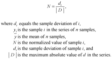 (2)
(2)
Long-term trend analysis was performed on three gaging stations in the Wood River Valley that have at least 20 years of record. Mean annual and monthly streamflow trends were analyzed, as well as 7-day and 30-day low-flow values for the period of record. The Base Flow Index (BFI), derived by a systematic method of calculating the volume of base flow for annual data, also was analyzed for any statistically significant trends. Long-term trends in precipitation and temperature were determined and were compared with streamflow data to account for anomalies.
Kendall’s tau was used to test for a significant trend for all of the flow statistics with all of the p-values provided in table 5. In addition, the magnitude of the trend was estimated using Sen’s Estimate of Slope, also provided in table 5. The Kendall’s tau nonparametric hypothesis test measures monotonic correlation strength between two datasets (Helsel and Hirsch, 1992). In these cases, the two datasets are the flow statistic (mean annual and monthly discharge, 7- and 30-day low-flow values, and the BFI) and time. A strong relation between data sets indicates an increase or decrease in flow over time. The calculated p-value is the probability that the null hypothesis (no trend in data) is in fact true; thus statistical significance increases as p-values decrease. Surface-water trends were judged statistically significant at the 90-percent confidence level.
The 7- and 30-day low-flow statistics were calculated using a process that combines the U.S. Environmental Protection Agency (USEPA) BASINS program (Aquaterra Consultants, 2006; U.S. Environmental Protection Agency, 2006), S-Plus statistical software (Insightful Corp., 2005), and the USGS statistical library for S-Plus. This process calculates the annual low flow from the minimum value of an n-day moving average of daily streamflow. The annual minima are then plotted over the period of record to identify long-term trends for that site.
The BFI is calculated as the ratio of the volume of base flow to the volume of total flow for a given time period. It was developed by the Institute of Hydrology of the United Kingdom (1980a, 1980b) in an attempt to standardize base-flow calculations for reproducibility. This method was further improved and automated by Wahl and Wahl (1988) for use on unregulated streams in the United States. Traditional calculations originally developed for this application are based on a 5-day interval local minima slope estimate. For this study, a longer duration interval was used to account for large spring runoff events in the snowmelt-dominated streams of the Wood River Valley that typically occur over a several week period.
BFI calculations are made by an algorithm that identifies local hydrograph minima at a user-defined interval. As initially developed for rainfall-dominated basins in the United Kingdom and Midwestern United States, the interval was taken at 5 days. Turning points are calculated by a three-point linear regression when a user-defined threshold slope is exceeded, commonly taken as 10-percent difference. The base-flow hydrograph is then created by connecting the turning points and integrating the area below the line.
The BFI calculations for the Big Wood River at Hailey gaging station data (13139510) were based on a 30-day interval over a year to identify base flow of a snowmelt-driven system as opposed to one dominated by rainfall. The Big Wood River near Bellevue (13141000) gage data used a 40-day interval for the BFI calculation and the Silver Creek at Sportsman Access (13150430) gage data used a 5-day interval. A shorter interval period, such as the default 5-day period, will introduce “false peaks” during springtime flows from melting snowpack for the Big Wood River gages. Although these longer intervals may lead to slight underestimation of base flow for the increased springtime runoff, it provides a consistent and reproducible approach for the analysis of long-term datasets.
To estimate water-level changes in the Wood River Valley aquifer system between historic and current conditions (2006), one map representing each set of conditions was needed. Historic or predevelopment conditions refer to the period before 1970 with a relatively stable population (fig. 3), water withdrawals, and consumption. However, this study uses ground-water level data from 1970 to1986 to fill spatial data gaps in the study area and to coincide with previous studies for comparison. For purposes of this report, partial development refers to the period including predevelopment conditions to 1986. Current (2006) conditions were based on water levels measured in 98 wells in the study area during October 23–27, 2006. Maps were constructed of partial development and October 2006 conditions for the unconfined and confined aquifers. These maps were then used to develop the maps showing water-level changes between the two time periods. In addition, streamflow was measured at 13 sites concurrently with the October 2006 water-level measurements to identify gaining and losing stream reaches. Finally, stream discharge and ground-water levels were analyzed for trends.
Historic ground-water levels used for the partial-development ground-water level maps were obtained from the USGS National Water Information System (NWIS) and the Idaho Department of Water Resources (IDWR) well-information and ground-water level databases. Water-level measurements stored in these databases were made at different dates throughout the year and over a range of years. However, there were insufficient ground-water level measurements during October of a single year to represent the entire Wood River Valley aquifer system. Therefore, it was necessary to use water levels from multiple years and months.
The decennial census data shown in figure 3 shows a relatively stable Blaine County population through 1970; ideally, water levels measured prior to 1970 would be used to construct a predevelopment map representing stable ground-water withdrawal and consumption rates. However, there are insufficient pre-1970 water-level measurements to adequately represent the entire Wood River Valley aquifer system. Consequently, water-level data collected as recently as 1986 was selectively used to expand map coverage into recently developed areas. Because these later water-level data were collected after significant development began, the conditions represented are more properly described as partial development. Despite this broad definition of partial development, historic data still were unavailable for some tributary canyons, and thus are not included on the partial development ground-water level maps. In addition, despite the desirability of comparing water levels collected in October of partial-development years to October 2006 levels, ground-water levels measured during August through December were used to construct the partial-development maps because an insufficient number of historic October measurements were available. The final set of historic ground-water level measurements contained historic (1952-1986) water levels for 242 wells: 206 wells in the unconfined aquifer and 36 wells in the confined aquifer (appendix A).
The compromises described here are often necessary in the analysis of past ground-water conditions. They are made assuming that monthly and annual water-level fluctuations were less than 10 ft prior to 1986, an assumption discussed in more detail in sections, “Estimating Water-Level Change” and “Annual and Long-Term Fluctuation of Water Levels.” Because streamflow in the area is intimately related to ground-water levels, it integrates upgradient ground-water conditions and is thus another indicator of water-table variation when used in conjunction with the maps. It should also be cautioned that, except where historic and October 2006 water-level measurements coincide, the maps of water-table change indicate broad conditions and may not be suitable for precise site-specific interpretation of change.
The 242 wells used for the partial-development maps were recorded in the NWIS database with elevation accuracies ranging from 0.01 to 20 ft, depending on whether the elevation was determined from topographic maps, level surveys from benchmarks, or Global Positioning System surveys. The IDWR well-information database does not contain elevation accuracies for the wells it contains. Elevations for the wells used to construct the partial-development maps were determined from 10-meter digital elevation models (DEMs) for all wells with an elevation accuracy greater than 1 ft. There were 26 coincident wells between the 2006 and partial-development ground-water levels. For these wells, the Global Positioning System (GPS) surveyed elevations were used. The 2006 surveying methods and accuracy are discussed in section, “Survey of Well Locations.”
The GPS-surveyed elevations, the NWIS-listed well elevations, and well elevations derived from 10-meter DEMs were compared for the 98 wells measured in October 2006 in order to qualitatively evaluate the accuracy of the water-level changes determined by the GIS methods used to generate the change maps (appendix A). Overall, the average difference between the DEM-derived elevation and the GPS-surveyed elevation of the 98 wells was smaller than the average difference between the NWIS-listed well elevation and GPS-surveyed elevation. The mean, median, and range for the GPS/DEM elevation comparison were 5.1, 2.8, and 26.8 ft, respectively. For the GPS/NWIS elevation comparison, the mean, median, and range were 15.3, 3.1, and 1,000 ft, respectively. The NWIS elevations had one obvious outlier. However, if the outlier is removed, then the mean, median, and range for the GPS/NWIS comparison for the remaining 97 wells are still greater than that of the GPS/DEM comparison. Of the 98 GPS-surveyed wells, 18 were listed in NWIS with elevation accuracies of 1 ft or less. The comparisons of just these higher accuracy elevations in NWIS with the DEM and GPS derived elevations resulted in the DEM comparison having a mean, median, and range of 1.7, 1.2, and 7.4 ft, respectively, which are larger than the NWIS comparison.
Water levels in 98 wells in the Wood River Valley study area were measured by personnel from the USGS during October 23-27, 2006. In non-flowing wells, ground-water levels were measured using either steel tapes or calibrated electric tapes. In flowing wells, water levels were measured with a calibrated digital pressure gage. Of the 98 wells, 10 wells were completed in the confined aquifer, and the remaining wells were completed in the unconfined aquifer.
Well locations were selected to represent ground-water levels throughout the Wood River Valley, but parts of the study area lacking wells are inadequately represented. Although an emphasis was made to find wells located in the tributary canyons in the northern part of the study area and the transitions of the canyons with the main Wood River Valley, these canyons often contained few available wells.
Elevations of the 98 wells were measured using a combination of real-time kinematic (RTK) and fast-static differential GPS-surveying techniques. Trimble 5700 and 5800 GPS systems were used for the surveying. In areas with poor satellite reception, a nearby location with good reception was selected, and a Topcon GTS-312 electronic total station was used to survey the well location relative to the GPS-surveyed location. GPS surveying data were processed with Trimble Geomatics Office software (Trimble Navigation Ltd., 2007), and any well that was surveyed using the total station was corrected to its proper GPS position.
Errors in the GPS fast-static surveying ranged from 0.02 to 0.26 ft horizontally and 0.05 to 0.52 ft vertically, with a mean horizontal error of 0.07 ft and a mean vertical error of 0.16 ft. The RTK survey method produced smaller positional precision errors. However, because each surveyed point originated from a fast-static surveyed position, these errors translated into the larger fast-static original position errors. Fast-static errors are a result of short measurement times, poor satellite reception due to areal obstructions (such as tree cover or narrow canyons), or lack of satellites available at the time of measurement. The fast-static technique was used in areas where RTK was not possible.
The October 2006 and partial-development ground-water level maps were produced using a geographic information system (GIS). The study area boundary was defined by using a DEM converted to a slope model to determine the transition from the adjacent bedrock hills (high slope values) to the flat portions of the valley filled with unconsolidated sediment (low slope values). This transition represents the approximate location of the boundary between the unconfined aquifer and the adjacent bedrock in the tributary canyons and the main valley. This location matches the approximate aquifer boundary defined by Moreland (1977) and Frenzel (1989), and the Quaternary alluvium boundary defined in Worl and Johnson (1995) and in Breckenridge and Othberg (2006).
The ground-water-level surfaces were created using a spline interpolator technique that includes barriers in order to incorporate the effects of aquifer boundaries along the narrow northern valley and tributary canyons (Environmental Systems Research Institute, Inc., 2007). The spline interpolator is a deterministic interpolator that creates a smooth surface that must pass through each measured value. It is ideal for smoothly varying surfaces such as a typical potentiometric surface. The output of the spline interpolator is a grid with an interpolated value at each cell except for those cells containing a ground-water-level measurement that is assigned the measured ground-water level. The cell size for the resultant grids is 10×10 m.
The spline interpolator was applied to the entire study area except in the vicinities of Warm Springs Creek on the October 2006 map and Trail Creek on the partial-development map. The spline with barriers interpolator did not provide hydrologically realistic results due to a lack of data in these two areas, so a tension spline interpolator was used instead. The resulting grids for each map were then combined to create one ground-water surface map. Contour lines were then created from the ground-water surface map for display purposes (pls. 1 and 2).
The tension spline technique includes a weight option that controls the amount of curvature in the interpolated surface between known ground-water level points and an option to determine the number of data points used in the calculation of each interpolated cell. The two areas in which the tension spline technique was utilized used high weights (value of 10), allowing for more variation in the output surface at a greater distance from the data points. The few data points available in these areas resulted in less control of the interpolated surface for the tributary canyons.
The confined aquifer was evaluated separately for the October 2006 and partial-development potentiometric-surface maps with ground-water level measurement data from wells completed in the confined aquifer. The tension spline interpolator was used to create these maps because the data is contiguous and no irregular barriers or boundaries isolate data points. The confined aquifer interpolations also used as many available data points as possible for the October 2006 potentiometric-surface map (due to the limited amount of data available) and used a weight option of 10. The partial-development potentiometric surface map was created using this same interpolator and settings.
Cells of the interpolated surfaces or grids are better controlled when the interpolated cell is surrounded by data points. The interpolator will evaluate cells if there are data points on only one side of the evaluated cell. This can have unpredictable results due to the lack of control over the interpolated cell. All sections of contour lines derived from interpolated cells that are surrounded by actual data points are displayed as a solid line, whereas the remaining contours are dashed to indicate this lack of control over the interpolated value of the grid cell. The potentiometric surfaces derived from wells completed in the confined aquifer are only defined for the areas between or surrounded by ground-water level data points because the full extent of the confined aquifer is not well known.
Water-level changes between partial-development and October 2006 ground-water maps were estimated by using a GIS to subtract the October 2006 water-level surfaces of the unconfined and confined aquifers from the partial-development water-level surfaces. The results are ground-water level change maps for the two aquifers showing changes in the water-table and potentiometric surfaces. Lines representing water-level change were then created from the resulting ground-water change surfaces—ground-water level declines are shown as negative values and ground-water-level rises are shown as positive values.
For the water-level change maps, any line that was within both the October 2006 and partial-development maps’ solid-line contour was displayed as a solid line. If the line occurs in an area where either the October 2006 or partial-development maps’ lines were dashed, then the water-level change map was dashed to indicate an interpolated value with less confidence.
As previously described in section, “Partial Development Ground-Water Levels,” historic data were not always available to match the exact timing of the October 2006 ground-water level measurement. Therefore, it was necessary to use measurements made August through December from 1952 through 1986 to augment the dataset. To evaluate the effect of natural annual and multi-year variation in ground-water levels on the water-level change maps, wells with multiple water-level measurements were analyzed to constrain probable variation. The maximum water-level range was calculated for a well with multiple water-level measurements for a single year during the 5-month period from August to December as well as the entire year. A well could have several water-level range calculations if it was measured multiple times during multiple years. The range of water-level measurements in wells vary from those measured only twice during the period of record to those measured multiple times in a single week.
Streamflow was measured at selected sites in order to evaluate the interaction between ground and surface water. Changes in streamflow between measurement points on a stream indicate whether the stream is gaining flow from ground-water discharge (an increase in flow between the stations) or if the stream is losing flow to ground-water and recharging the aquifer (a decrease in flow between the stations). Late October was selected for the mass-measurement of ground-water levels and streamflow because the irrigation season and related surface-water diversion typically ends by mid-October, and July–October usually are the driest months of the year. Consequently, streamflow from small tributary basins and the return flow from drains have ceased by late October.
During October 23-27, 2006, streamflow was measured at 13 sites: 7 on the Big Wood River, 3 on its tributaries, 1 on a diversion, and 2 on Silver Creek (fig. 4). However, during the week of October 23-27, 2006, a large number of tributary streams were still flowing into the Big Wood River, and many active diversions were still removing water for irrigation. Because of the large number of streams and diversions, not all inflows and outflows to the Big Wood River could be measured for discharge. Without measuring the discharge of each individual inflow and outflow, the comparison of flow between each measurement site is somewhat limited and accurate calculation of stream gains and losses is not possible for the entire river reach.
Measurements of discharge were made with a current meter using the general methods adopted by the USGS. These methods are described in USGS Water-Supply Paper 2175 (Rantz, 1982; Rantz and others, 1982) and the Techniques of Water-Resources Investigations of the United States Geological Survey (TWRIs), Book 3, Chapters A1 through A19 and Book 8, Chapters A2 and B2, which may be accessed at http://water.usgs.gov/pubs/twri/.

![]() U.S. Department of the Interior | U.S. Geological Survey
U.S. Department of the Interior | U.S. Geological Survey
URL: https://pubs.usgs.gov/sir/2007/5258
Page Contact Information: Publications Team
Page Last Modified: Thursday, 01-Dec-2016 19:56:21 EST
