Scientific Investigations Report 2007–5261
U.S. GEOLOGICAL SURVEY
Scientific Investigations Report 2007–5261
By Randell J. Laczniak1, Alan L. Flint1, Michael T. Moreo1, Lari A. Knochenmus1, Kevin W. Lundmark2, Greg Pohll2, Rosemary W.H. Carroll2, J. LaRue Smith1, Toby L. Welborn1, Victor M. Heilweil1, Michael T. Pavelko1, Ronald L. Hershey2, James M. Thomas2, Sam Earman2, and Brad F. Lyles2
1U.S. Geological Survey
2Desert Research Institute
A basic way to evaluate the occurrence and movement of ground water in an aquifer system is to develop a water budget accounting for the aquifer system’s inflows (recharge) and outflows (discharge). Water budgets may be developed for aquifer systems of any size, and for this study, water budgets were developed at the subbasin, HA, and study-area scales. Previous estimates of water budgets for HAs in the study area are summarized and compared to water-budget estimates developed for this study. Average annual recharge and ground-water discharge were estimated at the subbasin scale to develop a water budget for each HA. In addition, recharge and discharge estimates were summed for the entire study area and used to develop a study-area water budget. Differences in estimated recharge and ground-water discharge at subbasin and HA scales were used to evaluate intrabasin and interbasin ground-water flow, respectively.
During the 1960s and 1970s, the USGS in cooperation with the State of Nevada, completed a series of reconnaissance studies to evaluate the ground-water resources of Nevada. The results of these studies were published in a series of reports describing the water resources of Nevada by HA. Each report provides estimates for some or all major water-budget components and most provide estimates of average annual recharge. The reconnaissance reports all applied similar approaches for estimating recharge and discharge.
Annual recharge has been estimated for the 12 HAs in the BARCAS study area and published in numerous reports (table 5). Estimates of recharge presented in reconnaissance reports typically were based on a method developed by Maxey and Eakin (1949). The method originally was developed to estimate the recharge to 13 HAs in east-central Nevada and empirically relates recharge to annual precipitation by trial and error adjustments of the “recharge efficiencies” to generate a balance between estimated recharge and estimated discharge (Maxey and Eakin, 1949; Dettinger, 1989). Recharge efficiency is the percentage of total precipitation in the recharge-source areas of a basin that becomes recharge on a long-term average basis (Dettinger, 1989). The method assumes that higher altitudes receive greater precipitation and have a greater percentage of precipitation that becomes recharge (Eakin, 1966). Five precipitation zones were defined by this method from the Hardman (1936) precipitation map of Nevada. Recharge efficiencies, determined by balancing recharge and discharge, were associated with each of the five precipitation zones. Recharge to a basin was estimated from the precipitation rate for each of the five zones, applying the associated recharge efficiency, and summing these values to obtain the total recharge rate. The method has been applied to more than 200 basins in Nevada.
Ground-water discharge typically has been estimated using a volumetric calculation of ET from major areas of phreatophytic vegetation (table 6). In most of the HAs in Nevada, ground water is discharged by evaporation from free-water surfaces and soils, and transpiration by phreatophytes where the water table is at or near land surface (Eakin, 1962). Ground-water discharge estimates are based on maps that delineate distinct groupings of phreatophytes and moist soils in ground-water discharge areas and coefficients relating these groupings to ET or ground-water discharge rates. ET rates were determined from pan evaporation and lysimeter data, and ground-water discharge rates from ET rates were adjusted downward to remove the local precipitation component. Ground-water discharge for an HA was estimated by computing the product of the ground-water discharge rates and the corresponding area for a particular vegetation or soil moisture grouping, and integrating the products for all groupings in the HA. At the time of most reconnaissance estimates, the volume of water used for irrigation and self-supply was small and often was ignored in water-budget computations. Spring flow typically was not accounted for directly in the water budget but was indirectly accounted for because the total ET estimated or measured from a discharge area includes spring flow (Eakin, 1960). In some reconnaissance studies, ground-water discharge was not determined independently but was assumed to be equal to the Maxey-Eakin estimate of recharge.
Since publication of the reconnaissance studies, various statistical, geochemical, and numerical methods have been used to reevaluate basin-wide recharge (table 5). These methods commonly are variations on the Maxey-Eakin method and often have relied on a different precipitation map, more recent estimates of ground-water discharge (Nichols, 2000), or on statistical analysis of Maxey-Eakin results for selected HAs (Watson and others, 1976; Epstein, 2004). Additional methods to estimate recharge include chloride-mass balance (Dettinger, 1989), deuterium-calibrated water accounting models (Kirk and Campana, 1990; Thomas and others, 2001), a recharge-accounting model (Flint and others, 2004), and numerical simulation (Brothers and others, 1993a, 1993b; Brothers and others, 1994). For HAs in the study area, Nichols (2000) generally reports the highest recharge estimates; Watson and others (1976) generally report the lowest recharge, typically slightly lower than values reported in the reconnaissance reports.
For estimates of ground-water discharge (table 6), reported methods are variations on the Maxey-Eakin method of multiplying a ground-water discharge rate by the associated area of phreatophytic vegetation. However, technological advances such as the utilization of micrometeorological and remote-sensing methods have improved ground-based measurements and area-wide estimates of ET (Nichols, 2000).
The primary source of water recharging ground water underlying the study area is precipitation originating in the high mountains that border the broad, elongated valleys characteristic of the region (fig. 19 and pl. 4). In general, the higher the mountain range, the greater is the precipitation. The rate at which precipitation infiltrates through the surface and underlying rock to recharge the regional ground-water flow system depends on the permeability of the bedrock, local evapotranspiration, the permeability of the soil, and the amount of water stored in the soil. Because most bedrock in the region has low primary permeability, the rate of infiltration into mountain blocks is controlled by the rock’s secondary permeability created by the fracturing of consolidated rock and enhanced by dissolution.
The distribution of ground-water recharge and first-order estimates of recharge rates were developed using a regional-scale, recharge-accounting model. This recharge model provides a means for evaluating and comparing the processes, properties, and climatic factors that ultimately control the potential for recharge under differing hydrologic conditions (Flint and others, 2004). The Basin Characterization Model (BCM) accounts for all water entering and leaving grid cells to determine areas where excess water is available, and whether this excess water is stored in the soil or infiltrates downward toward the underlying bedrock. Depending on the soil and bedrock permeability, the BCM partitions excess water either as in-place recharge or runoff. Runoff can evaporate or recharge along the mountain fronts or through stream channel sediments at some distance downstream of the mountain front. The model is an updated and refined version of the BCM initially documented in Flint and others (2004) and was applied in this study to estimate potential annual in-place recharge and recharge from runoff for 1970–2004. Details of the updated and refined BCM as applied to the BARCAS study area can be found in Flint and Flint (2007).
The BCM is a mathematical deterministic water-balance method that integrates maps of geology, soils, vegetation, air temperature, slope, aspect, potential ET, and precipitation. The model uses many of these data sets and internal computations to estimate the distribution of precipitation (fig. 20), snow accumulation and snowmelt, potential ET, soil-water storage, and bedrock permeability. The distribution of precipitation was estimated using the Parameter-Elevation Regressions on Independent Slopes Model (PRISM; Daly and others, 1994). PRISM estimated precipitation was compared to measured precipitation at 155 stations in Nevada and Utah. Annual measured precipitation for these stations averaged 12 in. and was about 1 in. less than PRISM estimates. Differences between measured precipitation and PRISM estimates had a standard deviation of 4 in. Therefore errors resulting from using PRISM to distribute precipitation in the BCM were considered negligible.
The accuracy of other BCM-estimated parameter distributions also was evaluated, such as snow accumulation and snowmelt, runoff, and potential ET. Snow accumulation and snowmelt models were calibrated to mid-winter and late spring Moderate Resolution Imaging Spectroradiometer (MODIS) satellite data for 2000–2004 (Flint and Flint, 2007). BCM-simulated runoff and potential ET have been calibrated to measured data in previous studies (Flint and Flint, 2007). For example, simulated runoff was within 5 percent of measured discharge from the nine Arizona basins with between 10 and 35 years of streamflow records. Simulated potential ET was calibrated to 204 California Irrigation Management Information System (CIMIS) sites in California and 26 Arizona Meteorological Network (AZMET) sites in Arizona in 2006.
The BCM precipitation and recharge relation for 1970–2004 were extrapolated using regression analysis to estimate long-term average recharge for 1895–2006. Recharge during the 1895–2006 period was assumed to be representative of long-term recharge to the BARCAS area and differed from BCM results because annual precipitation for 1895–2006 was 5 percent less than for 1970–2004 (Flint and Flint, 2007). The long-term average recharge for 1895–2006 was estimated for each subbasin by relating annual recharge computed by the BCM for 1970–2004 to annual precipitation using a threshold-limited, power function (Flint and Flint, 2007). The threshold-limited, power function largely interpolated values because more than 98 percent of the annual precipitation volumes for 1895–2006 were within the range that was observed during the 1970–2004 precipitation period. This approach assumes that antecedent conditions from previous years do not affect annual recharge. This assumption may be inappropriate for predicting recharge in any given year but should minimally affect the estimate of a 112-year average.
Long-term recharge was calculated as the combination of in-place recharge and 15 percent of the potential runoff for each subbasin in the 12 HAs of the study area (pl. 4). Total long-term recharge is estimated at about 477,000 acre-ft and potential runoff at about 361,000 acre-ft (appendix A). Assuming that 15 percent of the potential runoff becomes regional ground-water recharge, about 530,000 acre-ft of the precipitation on average, annually recharges the ground-water flow system. The HAs contributing the greatest amount of ground-water recharge to the study area (68 percent) are Steptoe, Snake, and Spring Valleys (fig. 21). The ground-water recharge in these HAs averages more than 100,000 acre-ft annually. The estimated annual recharge for all other HAs ranges from about 4,000 acre-ft in Little Smoky Valley to 35,000 acre-ft in White River and Butte Valleys. Average annual ground-water recharge is less than 15,000 acre-ft for Cave, Lake, Little Smoky, and Tippett Valleys (appendix A; fig. 21). Even though White River Valley is relatively large at more than 1 million acres (12 percent of the study area), this HA only contributes 7 percent of the total recharge. The 12 HAs in the study area average 0.06 ft/yr of recharge to the regional ground-water system. HAs that received more than 0.06 ft/yr of recharge are dominated by high permeability carbonate rock.
The dominance of in-place recharge or runoff in an HA depends on a number of factors, including altitude, area, and the type of rock in the surrounding bedrock highlands. Even though in-place recharge is the primary recharge source for all HAs, some areas receive significantly high quantities of total runoff, and for a few basins, the quantity of total potential runoff is greater than the estimated annual ground-water recharge (fig. 21). BCM results indicate that the source of most ground-water recharge is in-place recharge at high altitudes in Cave, Lake, Snake, Spring, and Steptoe Valleys. This conclusion is supported by dissolved gas and stable-isotope data collected during this study from 15 sites (Victor Heilweil, U.S. Geological Survey, written commun., 2007). In contrast, BCM results indicate that the estimated total potential runoff is greater than the average annual ground-water recharge in Lake and Snake Valleys. Climate variability and the climate periods used in the analysis add uncertainty to the recharge estimates.
The accuracy of recharge estimates given in this report depends primarily on the validity of assumed hydrologic processes and on the associated uncertainty of input parameters to the BCM. Although the overall accuracy in estimates of volumetric recharge may be difficult to quantify, the estimates presented in this report are considered reasonable because the BCM is a physically based method and therefore scientifically defensible. The BCM incorporates spatially distributed moisture accumulation, soils, and geology that directly affect recharge magnitude and distribution. Hydraulic properties and geologic distributions undoubtedly are not perfect, but the BCM is conceptually correct.
BCM recharge estimates were derived by assuming that net infiltration is equal to in-place recharge and that topographic boundaries coincide with ground-water divides. Actual conditions may differ from these assumptions for some areas but the effect on average annual, regional recharge estimates likely would be minimal because the primary recharge areas occur along ranges entirely within the study area.
Data are limited for some input parameters used in the BCM. As a result, the uncertainties associated with these parameters may be a significant source of potential error for estimates of ground-water recharge, particularly for two parameters—the saturated hydraulic conductivity of bedrock and the associated volume of runoff that becomes recharge. The hydraulic conductivity estimates for bedrock are uncertain because of limited data on hydraulic properties in recharge areas, particularly on the properties and spatial distributions of fractures, faults, and fault gouge. Hydraulic conductivities used in the BCM span up to five orders of magnitude for the least permeable units (Flint and Flint, 2007, table 2). BCM-estimated recharge is relatively sensitive to changes in saturated hydraulic conductivity of bedrock because this parameter determines the partitioning of water between in-place recharge and runoff (Flint and Flint, 2007). Although the portion of runoff that becomes recharge varies significantly across Nevada (Flint and others, 2004), an assumed value of 15 percent is considered reasonable for areas of central Nevada dominated by in-place recharge; however, the uncertainty likely is greater in runoff-dominated areas. Previous investigations used percentages of recharge from runoff ranging from a low value of 10 percent in the Death Valley regional flow system in southern Nevada to a high value of 90 percent for the Humboldt regional flow system in northern Nevada (Flint and Flint, 2007). These percentages were therefore chosen as the endpoints representing the range of uncertainty for the recharge estimates shown in figure 22 (gray bars)—10 percent for the low end and 90 percent for the high end. As a result, the uncertainty in recharge estimates increases for basins such as Lake, Snake, and Spring Valleys where the potential runoff recharge exceeds the potential in-place recharge (figs. 21 and 22).
The long-term average recharge estimates are within the range of previous estimates except in Snake, Steptoe, and Tippett Valleys (fig. 23). In these three HAs, the recharge estimates are greater than or equal to the upper limit of the range of previous values likely resulting from the prevalence of high permeability carbonate bedrock in the highlands surrounding these HAs. Unlike the adjusted BCM estimates, most of the alternative methods used to estimate recharge neglect the effects of spatial variability in bedrock and soil permeability.
One such alternative method, used in several studies in Nevada, is the chloride mass-balance method for estimating ground-water recharge (Dettinger, 1989; Maurer and Berger, 1997; Russell and Minor, 2002; Mizell and others, 2007). Mizell and others (2007) recognized that the chloride mass-balance analysis provides a reconnaissance level estimate of recharge for 9 of 12 HAs in the study area. Recharge estimates could not be made in three HAs (Long, Tippett, and Newark Valleys) due to the lack of available chloride data. Because of limitations to this methodology as discussed by Dettinger (1989), the chloride-mass balance estimated average annual recharge is expected to be more uncertain than estimates made using the water-balance method.
Ground water discharges naturally from the study area through a combination of four primary processes— (1) spring and seep flow, (2) transpiration by local phreatophytic vegetation, (3) evaporation from soil and open water, and (4) subsurface outflow. Transpiration and evaporation are collectively referred to in this report as evapotranspiration (ET). Of these four processes, the first three occur at or near land surface directly from the discharge area and are the focus of this section. In addition to these natural discharge processes, water also can be removed or discharged from the ground-water flow system through the pumping of wells.
Estimates of average annual ground-water discharge for the various HAs are based on estimates of average annual ET developed for each of the major ground-water discharge areas. Estimates of ground-water discharge represent pre-development conditions. Springflow does not need to be accounted for directly in an ET-based estimate of ground-water discharge because water discharging from springs is either lost through ET or recharges shallow ground-water flow systems where it later is transpired by the local phreatophytes. Including total springflow directly in the total discharge estimate would in effect be double accounting of this flow. Moreover, ET-based estimates of ground-water discharge do account for discharge contributed by lateral inflow or by upward diffuse flow from the underlying regional ground-water flow system. Average annual estimates of ground-water discharge do not account for ground water pumped for irrigation, public supply, and other uses. Ground water exiting an HA or the study area as subsurface outflow is discussed in terms of the difference between the estimated mean annual recharge and mean annual ground-water discharge.
ET is the process that transfers water from land surface to the atmosphere both as evaporation from open water and soil and transpiration by plants. ET rates generally are affected by changes in the depth to the water table or in the moisture content of the soil. As water is removed by ET, the water table declines and soils dry. As water levels decline and soil moisture lessens, the vigor of phreatophytic vegetation decreases. Conversely, as less water is removed, the water table rises and soils moisten, and the vigor of the phreatophytic vegetation often increases. Changes in ET, the depth to the water table, and the extent and vigor of phreatophytic vegetation all are indicators of changes in water availability.
The volume of water lost to the atmosphere through ET can be computed as the product of the ET rate and the acreage of vegetation, open water, and moist soil that contribute water to the ET process. Past ground-water resource assessments have used this calculation to estimate ET from many major discharge areas in Nevada and Utah (Maxey and Eakin, 1949; Eakin and Maxey, 1951; Eakin, 1960, 1961, 1962, 1966; Rush and Eakin, 1963; Hood and Rush, 1965; Rush and Kazmi, 1965; Eakin and others, 1967; Glancy, 1968; Laczniak and others, 1999, 2001; Nichols, 2000; Berger and others, 2001; Reiner and others, 2002). Using this calculation, an average annual estimate of ET is computed by summing ET from all areas discharging ground water. The procedure, as applied in this study, delineates groupings of similar vegetation and soil-moisture conditions (ET units) within major discharge areas, and computes the annual ET from each ET unit within a discharge area. Average annual ET for an area, such as a subbasin or an HA, is estimated by summing the annual ET computed for each of the ET units present. Average annual ET estimates for each ET unit are computed by multiplying the acreage of the unit by an appropriate ET rate based on the unit’s vegetation and soil conditions. The associated acreage of each ET unit is determined through field mapping combined with an analysis of satellite imagery. ET rates were estimated from rates given in the literature and from data collected at micrometeorological stations established primarily in shrubland vegetation in White River, Spring, and Snake Valleys (Moreo and others, 2007).
Numerous studies have shown that the amount of water lost to the atmosphere from areas of ground-water discharge by evaporation and transpiration varies with vegetation type and density, and soil characteristics (Laczniak and others, 1999, 2001, 2006; Nichols, 2000; Berger and others, 2001; Reiner and others, 2002; DeMeo and others, 2003). In general, the more dense and healthy the vegetation and the wetter the soil, the greater is the ET. Many of these studies have used multi-spectral satellite imagery to identify and group areas of similar vegetation and soil conditions within major areas of ground-water discharge. Multi-spectral satellite imagery records digital numbers that represent the amount of incoming solar radiation reflected from the Earth’s surface at different wavelengths within the electromagnetic spectrum (Anderson, 1976, p. 2; American Society of Photogrammetry, 1983, p. 23-25; Goetz and others, 1983, p. 576-581). Delineations based on these spectral groupings that are intended to differentiate areas of similar ET often are referred to as ET units.
More recent studies have estimated ET from many discharge areas in Nevada using Landsat Thematic Mapper (TM) imagery to map ET units (Laczniak and others, 1999; Nichols, 2000; Berger and others, 2001; Nichols and VanDenburgh, 2001; Reiner and others, 2002; DeMeo and others, 2003). TM imagery has a resolution or pixel size of about 100 × 100 ft and includes six spectral bands. The moderate spatial and spectral resolution and the availability and cost of TM imagery are advantageous to mapping the different vegetation and soil conditions in ground-water discharge areas common to the study area. Ten ET units (table 7) have been mapped from TM imagery in the study area (Smith and others, 2007). These ET units were selected to represent the different vegetation and soil conditions in the study area where ground water is lost by ET to the atmosphere. The characteristics of each ET unit differs—ranging from areas of no vegetation, such as open water, dry playa, and moist bare soil; to areas of denser vegetation often dominated by phreatophytic shrubs, grasses, rushes, and reeds. Three of the ten ET units describe shrub dominated environments.
The method used to delineate ET units and their spatial distributions varied based on attributes specific to the ET unit of interest. For example, ET units whose spatial distribution varies significantly from year to year because of changes in climatic conditions are best delineated as an average distribution from multiple years of imagery. An example of a temporally varying ET unit is open water. The distribution of open water increases and decreases with changes in annual precipitation, whereas the distribution of shrubland is scarcely influenced by these same changes. Shrubland, grassland, meadowland, and moist bare soil ET units were delineated using modified soil-adjusted vegetation indices (MSAVI, Qi and others, 1994) and a tasseled cap transformation (Huang and others, 2002) computed from a single TM image (Smith and others, 2007). Dry playa, marshland, and open water ET units were delineated using a published land cover map (Southwest Regional Gap Analysis Program, SWReGAP) that was based on multiple dates of TM imagery (Kepner and others, 2005). And lastly, recently irrigated lands were delineated from multiple dates of TM imagery (Welborn and Moreo, 2007). The acquisition time of the TM images used in this analysis generally coincides with the near-peak period of ET around the summer solstice. The ET units delineated by the different techniques were combined in each ground-water discharge area and together form the ET unit map shown on plate 4. Additional details and the assessment of the overall accuracy of the mapped ET units can be found in Smith and others (2007).
Shrubland is the most prevalent ET unit in the study area (fig. 24, pl. 4). Shrubland, defined as the combined acreage of sparse, moderately dense and dense desert shrubland, occupies more than 80 percent of the acreage delineated as potentially contributing to ground-water discharge (Smith and others, 2007).
Prior to agricultural development, shrubland acreage was likely greater than accounted for in this study, considering that the ET units include irrigated cropland in areas likely to have been previously populated with phreatophytic shrubs and riparian vegetation (Smith and others, 2007). Riparian vegetation, such as marshland, meadowland, and grassland, occupies only about 6 percent and open water occupies less than 0.1 percent of the ET-unit acreage in the study area.
Shrubland occupies more than 60 percent of the ET-unit acreage within every HA (fig. 24), but percentages of the different density shrubland units vary from valley to valley. For example, Steptoe Valley has less sparse desert shrubland acreage than moderately dense shrubland, whereas in Snake Valley, sparse desert shrubland is the dominant ET unit. Other ET units occupy no more than about 20 percent of the total ET-unit acreage in any HA. Dry playa is prevalent only in Newark, Snake, and Spring Valleys (fig. 24). In Snake Valley, dry playa occupies nearly 65,000 acres of the valley’s ground-water discharge area.
HAs having ET-unit acreage exceeding 150,000 acres are Snake, Spring, Steptoe, and White River Valleys (fig. 24). Snake Valley has the greatest ET-unit acreage at nearly 330,000 acres. ET-unit acreage in Jakes, Little Smoky, and Tippett Valleys is less than 10,000 acres. Jakes Valley has the least ET-unit acreage at only 1,200 acres. In general, the larger the HA, the greater is the ET-unit acreage (pl. 4). The more densely vegetated ET units (meadowland and marshland) typically occur near springs and along major spring-drainage channels near the center of the valley floor. The less densely vegetated ET units, such as shrubland and grassland, typically occur along the outer edge of the discharge area or near the perimeter of the vegetation surrounding individual springs (pl. 4). For each HA, ET-unit acreage by subbasin is shown in figure 25. ET-unit acreages for individual subbasins used to develop the ground-water discharge estimates are given in appendix A and described in Smith and others (2007).
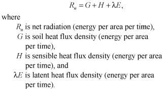
The rate at which water evaporates from the earth’s surface and is transpired by plants is referred to as the ET rate. The ET rate is driven by the available solar energy. Available solar energy is the difference between incoming and outgoing long and shortwave radiation. This energy difference is defined as net radiation (Rn, fig. 26). Net radiation is absorbed at the Earth’s surface, and then is partitioned into energy that is transferred by heat conduction downward into the subsurface, by heat conduction or convection upward into the atmosphere, or is used to convert water from the solid or liquid to vapor phase (Brutsaert, 1982). The partitioning process, which is governed by the conservation of energy and described by the surface energy budget, can be expressed mathematically as:
 (1)
(1)
The latent-heat flux component (λE) of the energy budget is the energy flux used for ET. Accordingly, ET can be calculated by subtracting the sensible heat (H) and soil heat (G) flux components of the energy budget from the net radiation (Rn, fig. 26). However, because this approach has been hampered historically by difficulties in measuring sensible-heat flux, a common solution to calculating ET has been the use of the Bowen ratio (Bowen, 1926). In simple terms, the Bowen ratio assumes that the proportionality between sensible and latent heat can be defined by the ratio between the temperature and vapor-pressure gradient. Because temperature and vapor pressure can be measured directly, the Bowen ratio can be substituted into the energy budget to solve for latent heat by directly using measurable parameters. Another technique used to estimate ET is the eddy-correlation method. Eddy correlation measures sensible- and latent-heat fluxes directly. Eddies are turbulent airflow caused by wind, the roughness of the Earth’s surface, and convective heat flow at the boundary between the Earth’s surface and the atmosphere (Kaimal and Finnigan, 1994).
A high-speed hygrometer and three-dimensional anemometer are used to measure sensible- and latent-heat fluxes carried by the turbulence in this boundary layer. These turbulent-type fluxes (H + λE) can be compared to available energy (Rn–G) to assess the performance of the eddy-correlation system. Over the last 25 years, many of the estimates of ET made in Nevada and the surrounding area have been based on one of these two methods (Carman, 1989; Nichols, 1993; Nichols and Rapp, 1996; Stannard, 1997; Laczniak and others, 1999; Nichols, 2000; Berger and others, 2001; Reiner and others, 2002).
ET rates depend on vegetation type, vegetation density, soil type, soil moisture, and local micrometeorological factors (Duell, 1990; Nichols, 2000; Berger and others, 2001; Laczniak and others, 2001). ET rates for different plant communities and soil type and moisture conditions have been measured across the Western United States for more than a hundred years (Nichols, 2000). Many early ground-water discharge estimates made throughout Nevada relied on ET rates measured elsewhere in the Western United States. Reports published from the 1940s through the 1970s (Maxey and Eakin, 1949; Eakin and Maxey, 1951; Eakin, 1960, 1961, 1962; Hood and Rush, 1965; Rush and Kazmi, 1965; Eakin, 1966; Eakin and others, 1967; Glancy, 1968) include estimates of ET rates that were based on measurements made over vegetation and soil similar to that found throughout the study area (Lee, 1912; White, 1932; Young and Blaney, 1942). ET rates reported in the more recent literature (Nichols, 2000; Berger and others, 2001; Reiner and others, 2002; Cooper and others, 2006) were used to develop a range of average annual ET for each ET unit inclusive of the variations associated with the different vegetation and soil-moisture conditions making up the ET units delineated for the study area. Annual ET estimates developed from reported values vary from less than 1 ft over playa and sparse shrubland units to more than 5 ft from open water areas (fig. 27).
Annual ET ranges for selected ET units were assessed and refined using field data collected at six eddy correlation sites deployed from September 1, 2005, to August 31, 2006. A typical site setup is illustrated in figure 28. Five of the six ET sites were located in the greasewood-dominated shrubland, and one was located in a grassland/meadowland area. The majority of the sites were located in shrubland to evaluate the effect of vegetation density on ET rates, and to better quantify ET rates for this dominant vegetation type. Daily and annual ET for the grassland/meadowland ET site (SPV-3) was significantly greater than that for shrubland ET sites in Spring Valley over the 1-year collection period (figs. 29 and 30).
The SPV-3 ET site represents an environment where annual ET far exceeds annual precipitation, and where ground water rather than precipitation serves as the primary water source supporting local ET. The SPV-1 ET site represents a typical shrubland environment, where measured ET barely exceeds precipitation, indicating that precipitation rather than ground water is the primary source of water consumed by ET (Moreo and others, 2007). ET measured over the 1-year collection period ranged from about 10 in. in sparse shrubland to 27 in. at the grassland/meadowland ET site (fig. 30).
The average annual ET for a discharge area can be estimated volumetrically as the product of the ET rate and the area over which ET is occurring. ET rates used to estimate average annual ET were assumed representative of the pre-development, long-term rates occurring in the study area. Therefore, the ET rate used to represent acreages in the discharge area defined as recently irrigated cropland (Welborn and Moreo, 2007) was replaced with a mixed phreatophytic ET unit that was assigned an ET rate that equaled the area-weighted average ET rate for all other phreatophyte units delineated in the study area.
Total ET estimated for a HA is the sum of its subbasin ET estimates (fig. 31). The subbasin ET estimate is the sum of ET estimates for each ET-unit. The ET estimate for an ET-unit is computed as the product of its ET rate and acreage (fig. 32). An ET-unit’s ET rate is determined by linearly scaling the ET-rate range computed for the unit (fig. 27, appendix A). Scaling within the range was done using the average MSAVI value for the unit computed over the subbasin from TM imagery. The scaling procedure assigns the highest average MSAVI value computed for any subbasin to the high value of the range and the lowest MSAVI value to the lowest value of the range. Details on the calculation and distribution of the MSAVI values used to scale ET rates are given in Smith and others (2007).
Annual ground-water discharge from HAs is computed as the difference between annual ET and local precipitation. Precipitation falling directly on ground-water discharge areas and surface-water run-on (overland flow) to discharge areas contribute to ET. Most precipitation falling directly on areas of ground-water discharge ultimately is lost by local ET, and therefore, is assumed not to contribute to ground-water recharge. In addition, most if not all surface-water flow onto fine-grained playa sediments evaporates, and for the purpose of the water budget is assumed not to contribute to either ground-water recharge or discharge. These assumptions are considered reasonable for these semi-arid valleys of the study area.
The average annual precipitation falling directly on ET units was estimated from a map of mean annual precipitation generated from model simulations of monthly precipitation distributions used to estimate average annual recharge for the BARCAS study area over the period 1970–2004 (Flint and Flint, 2007). Estimates of the average annual precipitation to discharge areas delineated within HAs range from about 6 in. in Little Smoky Valley to about 13 in. in Cave Valley (fig. 33, appendix A). In general, precipitation to discharge areas decreases from north to south. Contrarily, the highest annual precipitation occurs in Cave and Lake Valleys in the southern part of the study area. This anomaly is attributed to orographic effects. These effects also contribute to higher annual precipitation in the southern subbasins of Snake and Steptoe Valleys.
Annual ground-water discharge from HAs is the difference between annual ET and local precipitation, and ranges from only 860 acre-ft in Jakes Valley to 130,000 acre-ft in Snake Valley (fig. 31). Average annual ground-water discharge is estimated at more than 75,000 acre-ft in Snake, Spring, Steptoe, and White River Valleys, and at less than 10,000 acre-ft in Cave, Jakes, Lake, Little Smoky, Long, and Tippett Valleys. Combined ground-water discharge from Newark, Snake, Spring, Steptoe, and White River Valleys accounts for 95 percent of the estimated total annual discharge.
The proportion of the ET occurring as ground-water discharge generally decreases as the percentage of dry playa, sparse vegetation, or precipitation increases in the HA. That is, if the HA contains dominantly sparse phreatophytic vegetation or receives abundant precipitation, most of the local ET is more likely to be supported by local precipitation rather than by regional ground water. For example, in Little Smoky Valley about 55 percent of the average annual ET is supported by regional ground-water discharge, whereas in Long Valley, only about 10 percent of the average annual ET is supported by regional ground-water discharge. The discharge area for Little Smoky Valley consists of shrubland and some meadowland and grassland, and receives only about 6.3 in. of precipitation annually. In contrast, Long Valley’s discharge area consists wholly of shrubland and receives an average of about 11 in. of precipitation annually. The limited ground-water contribution to ET in Long Valley is a consequence of the valleys relatively high local precipitation.
The overall accuracy of the ground-water discharge estimates given in this report depends on the validity of the assumptions made in calculating volumetric discharges; and on any errors in estimates of ET-unit acreage and rate, and in estimates of the direct precipitation falling on an ET unit. The primary assumptions affecting the accuracy of average annual discharge estimates are:
The potential error resulting from any of these assumptions is not expected to significantly alter estimates presented in this report and was further evaluated in a detailed statistical analysis by Zhu and others (2007). Their analysis computes uncertainty stochastically using Monte Carlo simulations and compares differences in the uncertainty range computed for HA and subbasin discharge estimates. Standard deviations were used to define the uncertainty ranges shown in figure 34 for each HA discharge estimates.
Errors associated with estimates of ET-unit acreage largely depend on the quality and resolution of the multi-spectral imagery, on the appropriateness of the spectral technique used to delineate ET units, and on the accuracy of the boundaries used to depict the extent of phreatophytes in the study area. The MSAVI analysis of TM imagery used in this report, along with the inclusion of selected SWReGAP-delineated land classes, are assumed appropriate for identifying and delineating phreatophyte distributions for purposes of this report. An assessment of the accuracy of the delineated ET units is included in Smith and others (2007). The uncertainties defined by their assessment were used by Zhu and others (2007) to quantify the uncertainty associated with of the discharge estimates given in this report.
Shrubland, grassland, meadowland, and moist bare soil ET units were developed from a single set of images acquired in July 2005. Changes in the local vegetation can result from seasonal or annual increases or decreases in precipitation. These changes affect the vigor of the local vegetation, soil-moisture conditions, and the depth to the water table. Although imagery acquired near the summer solstice is considered reasonable for mapping phreatophytes in the study area, delineations certainly could be improved by using multiple years of imagery and multiple images within years. The inclusion of multiple images would provide more confidence in acreage estimates intended to represent long-term average ET rates. Errors in the ET rate are linked to any inaccuracies in reported values, and in potential errors associated with eddy-correlation measurements made in the study area. Uncertainty associated with the eddy-correlation technique, described in numerous publications and specifically addressed for this study in Moreo and others (2007), is expected to be less than about 10 percent. Because ET was computed from measurements made during only a 1-year period and at a limited number of ET sites, confidence in the degree to which these measurements represent average annual values and the average value over an entire ET unit would be improved with additional temporal and spatial data.
Estimates of average annual ground-water discharge are intended to account only for that ground water being lost to the atmosphere by ET, and are not inclusive of any springflow that leaves the discharge area by means other then by ET, or any subsurface outflow to adjacent basins. Without accurate measurements or estimates of these outflows, values given in this report should be considered minimum estimates of the total volume of ground water exiting an HA. Because ground-water discharge is estimated from ET, annual estimates of HA and subbasin ground-water discharge presented in this report include the surface runoff and streamflow that enters the ground-water flow system from areas outside of a discharge area.
Water is used for farming, mining, ranching, light industry, and domestic and public supply and is reported by water use, where each use describes the general application for which the water is used. Water uses were categorized as meeting irrigation and non-irrigation demands; the latter category includes public supply, domestic (self supplied), stock, and mining water use. Irrigation water use, the water-use class associated with the highest water consumption (89 percent of the total water demand), is estimated for 2005 on the basis of irrigated acreage delineated from multi-spectral satellite imagery and crop-application rates developed from climate data and known crop requirements. Estimates of non‑irrigation water use were reported by County, State, and Federal agencies responsible for regulating and planning current and future development.
Water withdrawn from wells or diverted from springs and mountain-front runoff in the study area is estimated at 126,000 acre-ft in 2005 (appendix A). Total water-use estimates for each HA range from less than 20 acre-ft in Cave and Tippett Valleys to 35,000 acre-ft in Snake Valley (fig. 35). Lake, Snake, Spring, Steptoe, and White River Valleys account for about 89 percent of the total water demand from the study area. Public supply, domestic, mining, and stock use were significant only in Steptoe Valley, where these uses accounted for about one-half of the total water demand. Combined stock and domestic uses accounted for less than 2 percent of total water demand.
Irrigated acreage was estimated from TM imagery using a procedure similar to that described in Moreo and others (2003). Details of the procedure are given in Welborn and Moreo (2007). More than 600 irrigated fields were mapped for 2000, 2002, and 2005 (figs. 36 and 37). Actively irrigated fields identified from the 2005 TM imagery were assessed for accuracy by site visits made during the 2005 growing season. Less than 5 percent of the fields identified as active were determined to be inactive during the field inventory, and accordingly, were removed from the 2005 acreage inventory. Delineated acreage was compared to available Nevada Division of Water Resources (NDWR) crop inventories. Total irrigated acreage estimated by both methods agreed within 9 percent in 2005 (Welborn and Moreo, 2007). Irrigated acreage for 2005 totaled 32,000 acres, ranging from less than 200 acres in Butte, Cave, Jakes, Long, and Tippett Valleys to 9,200 acres in Snake Valley (appendix A, fig. 38). Irrigated acreage increased about 20 percent from 2000 to 2005. Cave, Long, and Tippett Valleys essentially had no active irrigation throughout this period.
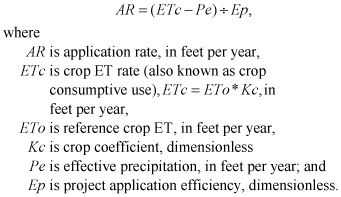
The application rate, or the amount of water that needs to be applied to each field to obtain maximum crop yield, depends on the length of the growing season, climate, prevailing management practices, and crop type (U.S. Department of Agriculture, 1993). A range for the likely application rate of each field was developed from the equation:
 (2)
(2)
Crop consumptive use is estimated as the product of reference crop ET and a crop coefficient assuming standard conditions. Standard conditions assume optimal field, environmental, and management conditions (Allen and others, 1998). Estimates of consumptive use, based on the crop coefficient method, are used extensively throughout the world (http://www.fao.org/nr/water/aquastat/water_use/index2.stm accessed May 9, 2007). ETo is a measure of the evaporative power of the atmosphere and can be computed from solar radiation, temperature, wind speed, and humidity (Allen and others, 1998). ETo was estimated by extrapolating rates for Nevada using more than 240 weather sites operated by the California Irrigation Management Information System (CIMIS; http://wwwcimis.water.ca.gov) and 26 weather sites operated in Arizona by the Arizona Meteorological Network (AZMET; http://ag.arizona.edu/azmet/) (Flint and Flint, 2007). The standardized Penman-Monteith reference equation is used by CIMIS to calculate ETo (Allen and others, 1998, 2005). ETo estimates for the study area average 2.8 ft/yr for the growing season (April-October) and 0.4 ft/yr for the non-growing season (Flint and Flint, 2007; Welborn and Moreo, 2007).
Kc relates crop consumptive use to the ETo rate, and depends on the growth and development of specific crops. CIMIS has developed Kc values specifically for calculating crop consumptive use as described above. For example, the average Kc is 1 for alfalfa during the growing season. Estimates of average crop consumptive use (ETc) for each HA, ranging from 2.78 to 3.08 ft/yr, are in agreement with measured consumptive-use rates for alfalfa and pastureland given in Maurer and others (2006) for a similar climate. Alfalfa and other hay production accounts for about 88 percent of the irrigated acreage in the study area. Pastureland accounts for about 10 percent, and corn, potatoes, and small grains account for about 2 percent of the total acreage irrigated in 2005.
Effective precipitation (Pe) is the amount of precipitation that remains in the root zone long enough to support crop growth. Factors such as precipitation amount, intensity, frequency and spatial distribution; topography and land slope; the depth, texture, and structure of the soil; depth to the water table; and water quality all affect Pe (U.S. Department of Agriculture, 1993). Pe is estimated to be 70 percent of the average annual precipitation and was estimated both for the growing and non-growing seasons because precipitation falling in the non-growing season increases the soil-water content, and any water retained in the root zone could be used for crop growth during the next growing season (U.S. Department of Agriculture, 1993). About two-thirds of the average annual precipitation falls during the growing season (Flint and Flint, 2007; Welborn and Moreo, 2007).
Project application efficiency (Ep) is the ratio of the quantity of irrigation water stored in the root zone to quantities of water diverted or pumped, and varies with the irrigation method and irrigation system used. Irrigation-system inefficiencies result from surface runoff or infiltration past the root zone, direct evaporation into the atmosphere, water intercepted at soil and plant surfaces, wind drift, and conveyance losses. Application efficiency is difficult to estimate accurately because the efficiency of an irrigation system is highly dependent on irrigator management decisions (U.S. Department of Agriculture, 1993). Because of these difficulties, Ep for the study area is estimated using standard published efficiency percentages (U.S. Department of Agriculture, 1993, 1997). After applying standard percentages, and field verifying irrigation methods and systems in the study area, Ep was estimated to range from 70 to 80 percent for center-pivot (continuously moving) sprinkler systems (fig. 39), from 55 to 70 percent for fixed and periodically moved sprinkler systems, and from 50 to 80 percent for the various types of flood irrigation systems. Fifty-three percent of irrigation applied in the study area is by center pivot sprinklers, 25 percent by fixed and periodically moved sprinklers, and 22 percent by flood irrigation (Welborn and Moreo, 2007).
Water withdrawn or diverted for irrigation is estimated as the product of irrigated acreage and an application rate estimated for each field. The average irrigation application rate for each HA ranged from 3.0 to 3.8 ft/yr (appendix A). Higher application rates reflect higher ETo rates, lower Pe rates, less efficient irrigation systems, or some combination thereof. The highest irrigation water use estimated for 2005 was in Snake Valley at 34,000 acre-ft (fig. 35). The uncertainty associated with irrigation water-use estimates is about plus or minus 15 percent based on the range of irrigation system efficiencies.
Irrigation return flow is that portion of the applied water that percolates beneath the root zone and ultimately returns to the ground-water flow system. Return flow is difficult to estimate because of the uncertainties in estimating application efficiency on a regional scale, travel time through the unsaturated zone, and the actual depth of the water table below the field. Stonestrom and others (2003) report travel times on the order of several decades for 8–16 percent of applied irrigation water to return to the saturated zone in the Amargosa Desert in southern Nevada. Return flow rates probably differ between flood and sprinkler methods because sprinkler irrigation systems lose an estimated 10–15 percent of applied water directly to evaporation and wind drift (U.S. Department of Agriculture, 1993). Given these uncertainties and limited available data, an irrigation return flow estimate of 50 percent of water available for return flow is considered reasonable. For example, applying equation 2 to a hypothetical 125-acre alfalfa field in Snake Valley irrigated with a center-pivot sprinkler system with Ep = 0.75, ETc = 3.0, and Pe = 0.45 ft results in an AR (application rate) of 3.4 ft. The product of irrigated acreage (125 acres) and AR (3.4 ft) is 425 acre-ft. If 375 acre-ft (125 acres × 3.0 ft) is required by the crop, then 425 acre-ft needs to be withdrawn from the well to satisfy crop requirements because of irrigation system inefficiencies. Fifty percent of the unused portion of water withdrawn from the well (425 acre-ft – 375 acre-ft = 50 acre-ft), or 25 acre-ft, is the estimated return flow.
Ground-water pumped from wells and diverted from valley springs accounts for an estimated 70 percent of the water used for irrigation in 2005. The percentage is based primarily on field proximity to irrigation wells, springs, and natural and manmade drainage features, and where available—NDWR crop inventories (Welborn and Moreo, 2007). Perennial and intermittent streams sustained by upland springflow and above-average snowmelt account for the remaining 30 percent of the irrigation water applied in 2005.
Public supply, self-supplied domestic, stock, and mining water use account for only about 11 percent of total water demand (appendix A). Public supply uses are metered and reported annually to the U.S. Environmental Protection Agency (USEPA) for inclusion in the Safe Drinking Water Information System (SDWIS) database (U.S. Environmental Protection Agency, 2004). Public supply estimates include water supplied by public water purveyors to households, commercial establishments, prisons, schools, and campgrounds. Of the 9,637 people estimated to live in the study area (GeoLytics, 2001), an estimated 5,825 permanent residents and an unspecified non-resident population (primarily tourists) were served by public supply (appendix A). Community populations served by public water supply systems were subtracted from the total population and the remaining population of 3,812 people was assumed to used a self-supplied domestic water system. The self-supplied domestic use was estimated using this population (3,812 people) and a water-use coefficient of 300 gallons per person per day was applied (Nevada Department of Conservation and Natural Resources, 1999). Hydrographic areas with very small populations were assumed to use 10 acre-ft for domestic use (appendix A). Stock water use for most HAs was estimated as 0.32 percent of irrigation water use (Nevada Department of Conservation and Natural Resources, 1999): however, this estimate was modified to account for valleys having stock wells but no irrigation or total livestock populations (U.S. Department of Agriculture, 1975, 2002). Mining water use typically is metered and reported annually to NDWR. Data obtained from NDWR indicate that mining water use was significant only in Steptoe Valley (appendix A).
Except for Snake Valley, ground-water discharge estimates for HAs are comparable with previous estimates, and generally are less than the median value of the range (fig. 40 and table 6) (Maxey and Eakin, 1949; Eakin and Maxey, 1951; Eakin, 1960, 1961, 1962; Hood and Rush, 1965; Rush and Kazmi, 1965; Eakin, 1966; Eakin and others, 1967; Glancy, 1968; Nichols, 2000). The range in previous estimate values defined for Snake Valley is based on only two estimates (table 6). Differences in published discharge values primarily result from differences in methodology, but the overall range also is affected by the number and type of discharge estimates used to define the range. For example, some of the estimates in previous studies do not correct for precipitation and use total ET as their reported estimate of ground-water discharge, and others include pumping in their estimate of total ground-water discharge.
Previous investigations estimated ground-water discharge from limited data and many estimates are not clearly defined. For example, early investigations estimated ground-water discharge in a basin (Maxey and Eakin, 1949) simply by delineating phreatophytic areas where depth to water was less than 50 ft and assuming average annual ground-water use of 0.1 ft (Jim Harrill, U.S. Geological Survey, retired, written commun., 2007). Nichols (1994) introduced new techniques for measuring evapotranspiration and quantifying ground-water discharge. Even with these advances, ground-water discharge estimates from Nichols (2000) were limited by less accurate micrometeorological equipment, few annual estimates of evapotranspiration, higher cost of satellite imagery, and less advanced remote-sensing technologies.
Annual ground-water discharge estimates were developed for this study using more advanced remote-sensing techniques for identifying and classifying vegetation, many more measurements of local ET and precipitation, and more robust and accurate micrometeorological equipment resulting in more accurate delineations of ground-water discharge areas and improved estimates of local ET rates. Annual ET, precipitation, and ground-water discharge have been measured at 6 sites in the study area and more than 40 additional sites around Nevada since 1995 (Laczniak and others, 1999; Berger and others, 2001; Reiner and others, 2002; DeMeo and others, 2003; DeMeo and others, 2006; Laczniak and others, 2006; Maurer and others, 2006; Thodal and Tumbusch, 2006; Westenburg and others, 2006). Mapping phreatophytes in Nevada is continuously improving as more imagery becomes available and as the quality of imagery improves. Additionally, unlike for earlier results, the uncertainty of annual ground-water discharge can be estimated because the uncertainty associated with each component term can be better quantified.
Differences in average annual recharge and discharge provide a surplus or deficit of water for each HA that is balanced, for systems under pre-development conditions, by ground-water flow entering or exiting a basin (interbasin ground-water flow). For example, ground-water inflow may be significant to HAs where large spring discharges and phreatophytic areas can not be sustained by local recharge. Conversely, ground-water outflow may be significant from HAs where recharge is high and relatively deep water levels and small or non-existent phreatophytic areas result in less local ET (Eakin, 1966; Mifflin, 1968). For this study, a water surplus or deficit for each HA was balanced by interbasin ground-water inflow or outflow. This approach has been applied in previous studies on ground-water budgets for HAs in Nevada (Harrill and Prudic, 1998; Nichols, 2000).
For most HAs, the estimated average annual recharge exceeds the estimated ground-water discharge by 20 percent or more (tables 5 and 6). The high recharge in Steptoe Valley annually exceeds pre-development discharge by more than 50,000 acre-ft, the largest surplus of water for any HA. Large annual water surpluses also occurs in Butte and Long Valleys, where average recharge annually exceeds average discharge by more than 20,000 acre-ft. Except for Snake, Newark, and White River Valleys, the annual recharge exceeds annual discharge in the remaining HAs, ranging from less than 1,000 to 18,000 acre-ft. Even though these surpluses are relatively small, the percent difference between recharge and discharge can be quite large. In Cave, Long, Jakes, and Tippett Valleys, the annual discharge is 20 percent or less than the annual recharge, indicating that most of the pre-development discharge exits these valleys as subsurface outflow to adjacent valleys.
In contrast to recharge-dominated HAs, pre-development discharge annually exceeds recharge in Newark, Snake, and White River Valleys. The average annual recharge is about 20 percent less than the average annual discharge in Newark and Snake Valleys. In White River Valley, the annual recharge is less than one-half of average annual discharge, resulting in an average annual water deficit of more than 40,000 acre-ft. This relatively large deficit in White River Valley indicates that water discharging from springs and by evapotranspiration on the valley floor must be supported, in part, by subsurface inflow from adjacent valleys.
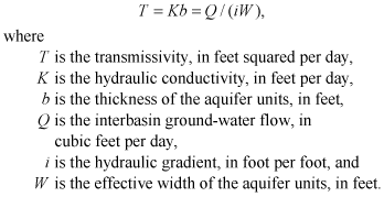
The potential for interbasin flow across HA boundaries is dependent on the magnitude of the surplus or deficit between average annual recharge and ground-water discharge, the transmissivity (the product of hydraulic conductivity and thickness) of aquifers along basin boundaries, and the hydraulic gradient of regional ground-water flow across basin boundaries. The magnitude of interbasin ground-water flow was estimated for all HAs in the study area using a water-budget accounting model, and these estimates were compared to estimates reported for previous studies, if available. For selected HA boundaries, estimates of the magnitude of interbasin flow were supported by evaluating transmissivity using the Darcy equation and by geochemical modeling.
A computer program documented by Rosemary Carroll and Greg Pohll (Desert Research Institute, written commun., 2007) was used to evaluate a water budget for the study area that included intrabasin and interbasin ground-water flow. The model, which is described by Lundmark and others (2007) is a single-layer representation of the regional ground-water system that accounts for quantities of ground-water flow across intrabasin divides and HA boundaries using a simplified mass-balance mixing model that utilizes deuterium as a conservative tracer. Deuterium values representing ground-water recharge and regional ground-water flow systems were based on existing and new data collected as part of the current study. These values were used as model input for recharge areas and to help calibrate the mixing model. A complete description of the spatial distribution and calculated average values for deuterium data model input and calibration can be found in Lundmark and others (2007).
Under pre-development conditions, the average annual recharge is greater than average annual discharge for 9 of the 12 HAs in the study area, indicating that a significant quantity of ground water must flow across intrabasin and interbasin boundaries. Intrabasin and interbasin ground-water flow, and flow to regions outside the study area, were: (1) constrained by the available volume of water (the difference between recharge and discharge estimates; pl. 4), (2) restricted to geologically and hydraulically suitable boundary segments, and (3) estimated using a deuterium-mixing model. Geologic barriers to ground-water flow are shown in figure 15. Hydraulic barriers to ground-water flow include relatively large areas of recharge creating mounds on the potentiometric surface and forming ground-water divides that separate the flow systems (pl. 3). The water-accounting model estimates quantities of ground-water inflow to, or outflow from, a HA but does not predict the location that ground-water flows across intrabasin or interbasin boundaries.
The accounting model was calibrated by approximately matching the simulated and measured deuterium concentrations and ground-water ET under pre-development conditions. For some HAs, model-predicted ground-water discharge rates were less than actual ground-water discharge rates estimated during this study. The differences were small, a few thousand acre-feet per year or less, and are considered to be within the uncertainty associated with interbasin flow rates. The details of the model are described by Lundmark and others (2007).
Model estimated interbasin flow rates and the general direction of flow across HA boundary segments are shown in figure 41. Butte, Cave, Little Smoky, Long, and Steptoe Valleys receive no ground-water inflow; Newark and Tippett Valleys receive only small amounts of ground-water inflow. The remaining five HAs, Jakes, White River, Lake, Spring, and Snake, receive ground-water inflow from adjacent HAs ranging from 20,000 to 80,000 acre-ft/yr. Ground-water flow out of the study-area boundary includes about 7,000 acre-ft/yr toward the north, from Steptoe Valley to Goshute Valley, and about 40,000 acre-ft/yr toward the northeast from Tippett and Snake Valleys to the Great Salt Lake Desert regional flow system. About 39,000 acre-ft/yr of ground water exits the study area to the south from White River Valley, providing water to the lower part of the Colorado regional flow system. About 8,000 acre-ft/yr exits the northwestern part of the study area from Butte Valley to the Ruby Valley regional flow system.
The model results represent a single solution that was obtained when the model was optimized to achieve a minimum difference between the simulated and measured deuterium concentrations and ground-water ET for the various HAs. However, model results are non-unique and other model simulations may yield similar residuals yet have significantly different flow patterns. Additionally, model-input deuterium values are sparse for several HAs, most notably Butte and Jakes Valleys. In addition to the uncertainty associated with a non-unique model and scarcity of deuterium data, the water-accounting model integrates information from multiple aspects of the study, including recharge and discharge estimates, and water-level data, each with its own inherent uncertainty.
Hydrologic and geochemical assessments were completed to support interpretations of intrabasin ground-water flow rates and locations based on results of the water-accounting model and associated hydrogeologic evaluations. The quantity of interbasin ground-water flow at selected HA boundaries was assessed indirectly using the Darcy equation. Geochemical modeling was applied to assess whether representative changes occur in the isotopic or chemical compositions of ground-water flow along paths that cross interbasin boundaries. These assessments do not provide independent estimates of the quantity of ground-water flow crossing interbasin boundaries, but are considered secondary evidence to support or refute the process of interbasin flow and provide general constraints on estimated flow rates.
Darcy’s Law was used to indirectly evaluate interbasin flow rates estimated by the water-accounting model. The law describes the relation between volumetric discharge or flow rate, ground-water flow gradient, cross-sectional flow area, and aquifer hydraulic conductivity or transmissivity (Freeze and Cherry, 1979). Transmissivity was calculated by dividing interbasin flow by the product of the hydraulic gradient and effective width of the interbasin boundary segment and formulated as:
 (3)
(3)
Transmissivity was estimated for six HA boundary segments and compared directly to aquifer test results given in Dettinger and others (1995). The interbasin flow values, cross-sectional areas, average thicknesses, hydraulic gradients, and corresponding hydraulic conductivity and transmissivity values for all boundary segments are shown in figure 42. Using equation 3, interbasin flow estimates from the water-accounting model (fig. 41) were used to calculate transmissivities. The hydraulic gradient across the HA boundary was estimated by calculating the ratio of the water-level difference and the distance between adjacent contour lines shown on the regional potentiometric-surface map (pl. 3). Aquifer widths were computed from cross sections extracted from a three-dimensional hydrogeologic framework model developed for this study (fig. 43).
Transmissivities were estimated for two HA boundary segments in the western half of the study area (segments A and B, fig. 42). Aquifer units beneath the shared boundary of Jakes and Long Valleys (segment A, fig. 42) and the shared boundary of Jakes and White River Valleys (segment B, fig. 42) include the upper carbonate unit (UCU) and the permeable conglomerates of the Diamond Peak Formation found in the upper half of the upper siliciclastic confining unit (USCU). The base of the ground-water flow system is assumed to coincide with the base of the conglomerates within the USCU. Transmissivity estimates of 66,000 and 150,000 ft²/d across segments A and B, respectively, are similar to estimates of Prudic and others (1995). The region used by Prudic and others (1995) is characterized as highly permeable.
Transmissivities were estimated for four HA boundary segments in the eastern half of the study area (segments C–F, fig. 42). The aquifer unit that underlies segments C, E, and F is the lower carbonate unit (LCU); whereas both the UCU and LCU aquifer units underlie segment D. The cross-sectional areas for boundary segments C and E are small (3 and 1 mi2, respectively) due to relatively short boundary segment lengths and shallow depths to the base of the flow system. The base of the ground-water flow system is defined at the subsurface contact with a detachment fault and top of the LSCU. The cross-sectional area of boundary segment F is 53 mi2 and the base of the flow system is relatively deep, coinciding with the top of the lower siliciclastic confining unit. The base of the flow system underlying segment D is unknown because each of the units, especially the UCU, likely contains numerous low-angle faults that may either disrupt the continuity of flow or promote brecciation of the rocks thereby increasing secondary permeability. The upper 0.6 mi of the LCU as well as the UCU are the aquifer units of interest underlying segment D. The transmissivities for segments C–F range from 1,400 to 5,800 ft²/d. The apparent differences in transmissivity between segments A and B in the western half of the study area and segments C, D, E, and F in the eastern half of the study area may correspond to the westward thickening of the UCU and LCU carbonate units and the coarsening of the intervening siliciclastic unit (USCU).
The calculated transmissivities for the various boundary segments can be compared with values for carbonate rocks presented in Dettinger and others (1995) (fig. 44). Transmissivity values for the entire carbonate-rock province range from 10 to 250,000 ft2/d. Based on aquifer tests at the seven wells located within or near the study area, the range is from 200 to 17,000 ft2/d (Dettinger and others, 1995).
All estimated transmissivities fall within the limits for permeable carbonate units in the carbonate-rock province (fig. 44). This comparison suggests that the interbasin ground-water flow rates estimated using the water-accounting model are consistent with the hydrologic properties of the carbonate rocks underlying the six boundaries considered here.
Geochemical modeling was applied to support other evidence of interbasin and intrabasin ground-water flow in the study area. Geochemical modeling focused on interbasin ground-water flow in the Spring Valley, Snake Valley, White River Valley, and Steptoe Valley HAs. These areas are the focus of the modeling because previous investigations (Harrill and Prudic, 1998; Nichols, 2000) concluded that ground water flows across boundaries between some of these HAs. Geochemical process models can be used to evaluate potential ground-water flow across HA boundaries or intrabasin divides by determining whether measured or inferred changes in the isotopic or chemical compositions of ground water along these proposed flow paths are possible. Geochemical processes include the dissolution or precipitation of minerals, input and loss of gasses, and ion exchange. Ground water at the beginning of a flow path may be representative of water from a single source area or from a mixture of waters derived from multiple source areas. A geochemical model also may include calculations of ground-water travel times—the time elapsed for ground water to move along a flow path between two locations. Although results from a geochemical model may support ground-water flow along a particular path by matching known chemical and isotopic compositions of the ground water, modeling results are not unique and are limited by knowledge of minerals and gases present in the aquifer and available geochemical data along potential flow paths (Hershey and others, 2007).
Ground-water flow paths that had reasonable major-ion and conservative tracer mixing relations were modeled geochemically using the computer program NETPATH (Plummer and others, 1994). The reasonableness of major-ion and conservative tracer mixing was assessed graphically (Hershey and others, 2007). NETPATH was used to interpret net water-rock mass-balance reactions between initial and final water compositions along a proposed ground-water flow path. Geochemical modeling results including ratios of initial and recharge waters (given as a range in percent) are summarized in table 8. Numerous valid water-rock reaction models for many of the flow paths were possible; for example, percentage of initial and recharge waters used for the two model evaluations along the flow path from northern Spring Valley to northern Snake Valley was 30 and 70 percent in the first evaluation (upper mixture, table 8), and 0 and 100 percent in the second evaluation (lower mixture, table 8). “Initial water” is water in springs or wells found at the beginning of the main flow path; “recharge water” is water from subsurface inflow of higher altitude springs tributary to the main flow path that potentially can be mixed with initial water. Details on chemical sampling, geochemical data, and results of NETPATH model evaluations on geochemical reactions and calculated travel times are provided in Hershey and others (2007).
Results of geochemical modeling support ground-water flow across selected HA boundaries, including ground water flowing (1) east from northern or southern Spring Valley into northern or southern Snake Valley, respectively, (2) southeast from southern Steptoe Valley to Spring Valley, and (3) southeast from Lake Valley to southern Spring Valley (fig. 45). Model results also support ground-water flow across selected intrabasin divides, including ground-water flowing north and south from central Spring Valley, and south from northern White River Valley into southern White River Valley (table 8). Moreover, chemical and isotopic data indicate that most of the ground water in Spring Valley originates as recharge in the surrounding Schell Creek and Snake Ranges, and that the Snake Range also is a major source of ground water in Snake Valley. Geochemical model could not be validated for other basins in the BARCAS study area due to lack of available chemical and isotopic data (Hershey and others, 2007). All geochemical models supporting ground-water flow across HA boundaries required some portion of local recharge along the flow paths. A detailed description of NETPATH-modeling results, including associated ground-water flow travel times and velocities can be found in Hershey and others (2007).
No single report presents estimates of interbasin ground-water flow for all HAs included in the BARCAS study, but several previous studies have reported on ground-water flow for multiple basins in the study area, or have been completed for a single basin in the study area (table 9). Nichols (2000) and Thomas and others (2001) report interbasin flow estimates for 8 and 5 of the HAs in the study area, respectively. Harrill and others (1988) present reconnaissance-level estimates for all HAs in the study area. Their estimates were based on locations, volumes, and directions of interbasin flow compiled from reconnaissance reports that generally represent evaluations of single HAs.
The interbasin flow estimates presented in Nichols (2000) assumed that (1) differences between recharge and discharge were equal to the interbasin ground-water flow into or out of the HA, and (2) the system is in hydrologic equilibrium such that discharge combined with interbasin flow can be used as a surrogate for recharge (Nichols, 2000, p. C21). Excess or deficient recharge for a given HA was compensated by interbasin flow into or out of the area if these flows were proposed in earlier studies or were otherwise permissible, geologically and hydrologically. Nichols (2000) found that the interbasin flow volumes were consistent with, and tended to corroborate most of the boundaries defined by Harrill and others (1988).
Interbasin flow volumes and assumed ground-water flow directions also were evaluated by Thomas and others (2001) using a deuterium mass-balance model. The deuterium data used to construct their mass-balance models are primarily historical data from DRI and USGS reports and databases. Estimated recharge to a valley and inflow from adjacent valleys were validated using deuterium data from regional springs and wells. Boundary conditions and input to their model were based on prominent geologic structure, stratigraphic continuity, and hydraulic gradients described in previous studies (Eakin, 1966; Thomas and others, 1986; Kirk and Campana, 1990; Dettinger and others, 1995; Thomas and others, 1996). Where recharge and ground-water inflow into a basin exceeded ET, excess ground water was assigned as subsurface flow to the next downgradient valley (Thomas and others, 2001). The model developed by Thomas and others (2001) is similar to the accounting model used in the current study, in that both models are modified versions of a deuterium mass-balance model originally developed by Campana (1975). However, these two models differ in a number of aspects, including their conceptualization of the aquifer system, model input values of recharge and hydraulic head, and spatial distribution and concentrations of deuterium data used to calibrate each model.
Directions of interbasin flow presented in Harrill and others (1988), Nichols (2000), and Thomas and others (2001) are in general agreement. However, the magnitude of interbasin flow differs slightly between reports. The primary directions of flow in the study area are (1) from north (Long Valley) to south (White River Valley) in the Colorado regional flow system; and (2) toward the north-northeast from Steptoe, Tippett, and northern Snake Valleys in the Great Salt Lake Desert regional flow system. Interbasin flow in these reports also was described as flowing southwest to Railroad Valley, northwest to Clover and Ruby Valleys, and east from Spring Valley, through Snake Valley, and into western Utah.
In general, interbasin ground-water flow directions described in this report are similar to those reported in previous studies for the Colorado and Great Salt Lake Desert regional flow systems. However, based primarily on interpretations of HA boundary geology, regional ground-water gradients, and water-accounting modeling, some interbasin flow directions discussed in this report differ from previous studies (fig. 41). For example, outflow from southern Steptoe Valley to Lake Valley, from southern Steptoe Valley to Spring Valley, and from Lake Valley to Spring Valley have not been postulated or are of much greater rates compared with previous studies. Based on regional flow systems defined by Harrill and others (1988), these interbasin flow directions occur across the boundaries of the Goshute and Colorado regional flow systems (Steptoe to Lake Valleys), of the Goshute to Great Salt Lake Desert regional flow systems (Steptoe to Spring Valleys), and of the Colorado to the Great Salt Lake Desert regional flow systems (Lake to Spring Valleys).
In most cases, BARCAS interbasin flow estimates are higher than previously reported with only a few estimates falling within the range defined by previous estimates in the study area (fig. 46). BARCAS inflow estimates are higher in Jakes, Lake, Tippett, Snake, Spring, and White River Valleys than previous estimates; and in Newark Valley, estimated inflows are near the middle of the range of previous estimates. BARCAS ground-water outflow estimates are significantly higher than published estimates in Spring and Steptoe Valleys, and moderately higher in Lake and Jakes Valleys. In Butte, Long, and White River Valleys, the estimated outflows are within the range of published estimates, and in Snake and Cave Valleys, the outflows are lower than published estimates (fig. 46). A Monte Carlo uncertainty analysis of the interbasin inflows and outflows was conducted as part of the steady-state water-budget accounting modeling effort. Results of the analysis are based on thousands of simulations and identify the 95-percent confidence interval for net interbasin inflow to and outflow from each of the hydrographic areas as well as for flow between subbasins. The 95-percent confidence intervals (error bars) for net interbasin flow are shown in figure 46.
Interbasin flow estimates may have a substantial amount of associated uncertainty because the accounting model integrates data from multiple aspects of the BARCAS study. This uncertainty is an accumulation of the associated uncertainty from the representation of the regional potentiometric surface, interpreted hydrogeologic boundary classifications, and recharge and discharge estimates. Moreover, deuterium data used in the model are relatively sparse in parts of the study area (Lundmark and others, 2007). The potential error and relative uncertainty has been evaluated and described in detail by Lundmark and others (2007).
Differences between estimates given in this study and in previous reports primarily are attributed to variations in the applied methods. For example, some previous estimates neglected hydraulic connections between adjacent HAs and, as a result, inflow from upgradient areas was not considered when constructing the water budgets. Additionally, discharge estimates from previous studies tend to equal the low end of the range for many of the individual HAs. This larger difference between recharge and discharge components suggests that larger volumes of ground water may be available for interbasin flow from recharge-dominated HAs to adjacent HAs. The greater estimated outflow from some HAs is considered reasonable because the study area is a primary recharge area for the Colorado, Great Salt Lake Desert, and Goshute Valley regional flow systems (pl. 3 and fig. 41).
Average annual recharge and ground-water discharge for HAs were summed and compared to evaluate the water budget for the study area, referred to in this report as the regional ground-water budget. Based on estimates for HAs, average annual ground-water recharge to the study area totals about 530,000 acre-ft, and average annual ground-water discharge totals about 440,000 acre-ft (appendix A). Assuming that these estimates represent pre-development conditions, the difference between estimated recharge and discharge indicates that about 90,000 acre-ft of ground water exits the study area annually as subsurface outflow. An outflow of this magnitude from the study area is not unexpected, considering that the area serves as the headwaters of two regional flow systems, the Colorado and Great Salt Lake Desert systems. Assuming that subsurface outflow supports these large regional flow systems, the likely major pathways for outflow are through Snake Valley to the northeast and White River Valley to the south (fig. 41). Ground-water outflow to the northeast from Tippett Valley also flows toward the terminal discharge area in the Great Salt Lake Desert flow system. Other major areas of ground-water outflow include the northern boundaries of Steptoe and Butte Valleys (fig. 41).
The net amount of regional ground water removed from the study area was estimated to evaluate the significance of the ground water withdrawn to ground water discharged under pre-development conditions. Net ground-water use represents the estimated amount of ground water pumped from wells or diverted from regional spring sources minus any water recharging the ground-water flow system as a result of water returned from mining, irrigation applications, or public supply. In making this estimate, local spring and surface runoff sources are assumed to account for 30 percent of the water-use estimates given in figure 35, and return flow as 50 percent of any unconsumed water. Net regional ground-water use estimated for each of the HAs in the study area ranged from near zero, primarily in unfarmed valleys, to nearly 24,000 acre-ft in Snake Valley; and in all HAs, are substantially less than the total water-use estimates (figs. 35 and 47). Net regional ground-water pumpage is greater only in Lake Valley than the estimated average annual ground-water discharge under pre-development conditions. Net regional ground-water use for the entire study area is estimated at about 80,000 acre-ft, or about 60 percent of the 2005 water-use estimate.
When including the estimated net ground-water use for 2005 in the regional water budget, the recharge and discharge components of the ground-water budget are nearly balanced over the entire study area—average annual recharge (530,000 acre-ft) is approximately equal to average annual ground-water discharge under pre-development conditions (440,000 acre-ft) plus estimated net ground-water use for 2005 (80,000 acre-ft). That is, the estimated net 2005 ground-water use is nearly equal to the estimated average annual ground-water outflow from the study area (90,000 acre-ft). On a regional scale, this condition suggests that the long-term use of ground water at about the 2005 estimate could capture the estimated average annual volume of ground water exiting the study area. Moreover, this condition also could, in some combination, decrease subsurface outflow, decrease spring discharge, decrease phreatophytic discharge, or increase subsurface recharge from adjacent basins. However, actual decreases in the volume of ground-water outflow, or in the volume of other pre‑development discharge components such as interbasin flow, spring discharge, or evapotranspiration, would be controlled by a number of factors, particularly, the spatial distribution of ground-water withdrawals, and the volume of ground-water removed from storage. For example, decreases in outflow would be less likely in Butte or Tippett Valleys where net ground-water use was zero in 2005 (fig. 47). Decreases in outflow would be more likely in subbasins having both high pumping and relatively large outflow such as in Snake Valley where net ground-water use was 24,000 acre-ft in 2005 and average annual ground-water outflow was estimated at 29,000 acre-ft (fig. 47). Additionally, the relatively large volume of water stored in the basin-fill aquifer (appendix A) would likely inhibit near-future decreases in ground-water outflow or in other pre-development discharge components if withdrawals are taken from the basin-fill aquifer. For example, water-level measurements show declines around major areas of pumping indicating that storage currently (2005) is a primary source of pumped ground water in the study area. Moreover, historical pumping has been periodic and often used only as a supplement to spring and surface sources. Ground-water pumping in prior years was substantially less than that estimated in 2005, and much of the current pumping occurs outside major discharge areas. Ongoing pumping has not yet significantly altered ET rates, regional springflows, or distribution of native vegetation. Evaluation of the timing and location of potential decreases in pre-development ground-water discharge would be best accomplished through the application of a numerical ground-water flow model; however, the development of a regional model was beyond the scope of the current study.
Some uncertainty exists on estimated differences between average annual recharge and pre-development discharge. These estimates were made independently, and each methodology has inherent limitations and associated uncertainty. Recharge estimates were model-derived; the accuracy of these estimates depends on the accuracy with which a number of hydrologic, atmospheric, and soil parameters were estimated. Estimates of pre-development discharge primarily were derived through field measurements and, as a result of a more direct method of measurement, the uncertainty of estimated pre-development discharge likely is less than the uncertainty of estimated recharge. Future studies may reduce uncertainties of estimated recharge and discharge by evaluating a regional ground-water flow system bounded by ground-water divides, such as the Colorado or Great Salt Lake Desert regional flow systems. Evaluating entire regional flow systems provides the constraint that ground-water inflow and outflow across the study area boundary is minimal; therefore, cumulative recharge and pre-development discharge must balance for HAs within the regional flow system.

![]() U.S. Department of the Interior | U.S. Geological Survey
U.S. Department of the Interior | U.S. Geological Survey
URL: https://pubs.usgs.gov/sir/2007/5261
Page Contact Information: Publications Team
Page Last Modified: Thursday, 01-Dec-2016 20:00:06 EST
