Scientific Investigations Report 2008–5025
U.S. GEOLOGICAL SURVEY
Scientific Investigations Report 2008–5025
Logistic regression was selected for this analysis because logistic regression quantifies the relation between a variable of interest (response variable) and one or more variables that affect the variable of interest (explanatory variables). This is conceptually similar to multiple linear regression. However, the response variable in logistic regression is transformed into a binary response (yes or no) variable. This makes logistic regression an excellent tool for modeling aquifer vulnerability to nitrate contamination because logistic regression can quantify the probability that nitrate will exceed a specified concentration. According to Tesoriero and others (1998),
“Logistic regression may identify relations between the occurrence of a constituent and explanatory variables when other methods do not because logistic regression answers a simpler question—whether a well is expected to have water with a concentration greater than a specified value. In contrast, other methods (e.g., linear regression) try to estimate the absolute concentration of a constituent. Given the many factors related to the source and transport of a constituent in ground water, it is often impossible to predict its concentration; however, it may be possible to predict the probability that the concentration is above a specified level.”
In this study, logistic regression models were used to determine the probability of exceedance of 2 mg/L of nitrite plus nitrate as nitrogen in ground water. For the models, a binary response variable was defined by dividing the measured nitrate concentrations into two groups: those greater than or equal to 2 mg/L (exceedances) and those less than 2 mg/L (nonexceedances). The threshold of 2 mg/L was selected because nitrate concentrations that exceed 2 mg/L generally are the result of anthropogenic effects (Nolan and others, 1998).
The logistic regression models take the form of
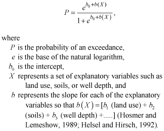 (1)
(1)
When the probability of an exceedance is plotted versus an explanatory variable, the result is an S-shaped curve with the probability being bounded by 0 on the lower end and 1 on the upper end. The SAS statistical software was used to determine (calibrate) values of b0 and b that best fit the data using an iteratively reweighted least-squares algorithm (SAS Institute, 1990).
Model performance was evaluated using several statistical measures. Logistic regression calculates several statistical parameters that determine the predictive success of the model. The log-likelihood ratio measures the success of the model as a whole by comparing measured with estimated values (Hosmer and Lemeshow, 1989); specifically, it tests whether model coefficients of the entire model are significantly different from zero. The most significant model is the one with the highest log-likelihood ratio, taking into account the number of explanatory variables (degrees of freedom) used in the model. The log-likelihood ratio can be approximated by a chi-squared distribution, and the computed p-value reflects the degree of certainty (significance level) that model coefficients as a whole are different from zero. A p-value of 0.05 indicates a significance level of 95 percent, a p-value of 0.01 indicates a significance level of 99 percent, and the smallest p-value indicates the best model. McFadden’s rho-squared (SPSS, Inc., 2000) is a transformation of the log-likelihood statistic and is intended to mimic the R2 metric of linear regression. Rho-squared is always between 0 and 1; a rho-squared closer to 1 corresponds to a better fit. Rho-squared tends to be smaller than R2, so a small number does not necessarily imply a poor fit. Values between 0.2 and 0.4 indicate good results (SPSS, Inc., 2000). The percentage of correct responses is a measure of how many actual nitrate exceedances and nonexceedances are present, compared with what was estimated by the model; the largest number denotes the best model. The percentage of correct responses is calculated as the number of measured exceedances estimated by the model as exceedances, plus the number of measured nonexceedances estimated by the model as nonexceedances, divided by the combined number of measured exceedances and nonexceedances (Nolan and Clark, 1997). Additional information regarding these statistical measures is available in Hosmer and Lemeshow (1989) and Helsel and Hirsch (1992).
The partial-likelihood ratio was used to compare nested models to determine the significance of adding one or more new variables (Helsel and Hirsch, 1992; Nolan and Clark, 1997). A nested model contains all explanatory variables in the original model, plus one or more additional explanatory variables. To determine whether the model is improved by adding the explanatory variable, the logistic regression model is calculated without that new variable. Logistic regression calculates a partial-likelihood ratio. The logistic regression model then is rerun with the additional new explanatory variable; the second model also calculates a partial-likelihood ratio. The difference in partial-likelihood ratios between the two models is calculated and a chi-squared approximation is calculated with degrees of freedom equal to the number of additional variables in the new model. If the p-value from the chi-squared distribution is less than 0.05, the model has been significantly improved at the 95-percent level.
For individual explanatory variables, the p-value for the Wald statistic is reported. The Wald statistic can be approximated by a chi-squared distribution and is used to indicate whether individual model coefficients are significantly different from zero. Individual coefficients were considered to be statistically significant if the p-value of the Wald statistic was less than or equal to 0.05. The p-value for the Wald statistic can be considered similar to the p-value for the slope of a line in linear regression. In linear regression, the slope of the line is considered to be statistically different from a horizontal line (with a slope of zero) if the p-value is less than 0.05. Similarly, the regression coefficients are considered to be statistically different from zero if the p-values are less than 0.05.
Multicollinearilty is the result of strong correlation between explanatory variables, and is a major concern for multivariate logistic regression models. Multicollinearity may result in incorrect signs and magnitudes of regression coefficients, thereby, leading to incorrect conclusions about relations between explanatory and response variables. Pearson correlation coefficients and multicollinearity diagnostic statistics were examined to assess the multicollinearity in the models. A strong correlation between two variables was indicated if the correlation coefficient was greater than 0.7. However, Pearson correlation coefficients would not detect cases where multiple explanatory variables may be interdependent. In these cases, the Tolerance and Variance Inflation Factor (VIF) can be used to detect multicollinearity. According to Gurdak and Qi (2006), the Tolerance and VIF are based on linear regression analysis of explanatory variables. The Tolerance is defined as 1 – R2, where R2 is the coefficient of determination for the regression of one independent variable on all remaining independent variables (Allison, 1991; Menard, 2002). The VIF is equal to the reciprocal of the tolerance and describes how inflated the variance of coefficient is compared to what it would be if there were no multicollinearity (Allison, 1991). Although no formal thresholds exist to use for the Tolerance or VIF in detecting the presence of multicollinearity, Allison (1991) suggests that Tolerance values less than 0.4 (VIF greater than 2.5) may indicate the presence of multicollinearity.
The binary response variable of nitrate concentrations exceeding or not exceeding a selected concentration (exceedances and nonexceedances, respectively) was computed from the WDOH public-water supply system database. The WDOH dataset contained more than 60,000 nitrate analyses from samples collected between April 1979 and September 2006. Because nitrate concentrations and land-use characteristics would be expected to have changed over such a long period, the dataset was reduced to include only the samples collected after January 1, 1995. Reporting level limits in this smaller dataset ranged from less than 0.001 to less than 7 mg/L. Because the wide range of reporting levels would adversely affect the computation of the response variable, analyses with reporting levels greater than 0.5 mg/L were omitted, which resulted in the exclusion of about 850 samples.
Once the dataset of nitrate analyses was finalized, a single nitrate concentration was calculated for each water source, as many of the sources had multiple samples. This was accomplished by computing the median value of all samples for each water source. The resulting dataset then was further reduced to exclude all water sources that were not from an individual well, had no location information, or had location information of questionable quality. The final dataset contained median nitrate concentrations for about 12,600 wells.
The final dataset contains far fewer wells in eastern Washington than in western Washington, but nitrate concentrations were elevated in a larger percentage of wells in eastern Washington (fig. 3). Nitrate concentrations were higher in wells in the Columbia basalt flow and the eastern Washington unconsolidated hydrogeomorphic regions than the other regions of the State (fig. 4). The regional median nitrate concentrations ranged from 1.4 mg/L in the eastern Washington alluvial fill region to the reporting limit of 0.5 mg/L in the western Washington alluvial fill, bedrock, and Puget lowland regions.
Nitrate concentrations in ground water from wells in the USGS and Washington State Department of Ecology databases (fig. 5) were used as the model validation dataset (1,813 wells). Only data collected after 1995 were used, and all known public-supply well samples were excluded so no data were duplicated in the calibration dataset. As with the calibration dataset, nitrate concentrations in the validation dataset were elevated in a larger percentage of wells in eastern Washington.
Explanatory variables that were compiled and evaluated included well depth (depth to bottom of well from land surface), ground-water recharge rate, average annual precipitation, population density, land use, nitrogen application amounts, soil available water capacity, soil hydrologic group, soil drainage group, soil permeability, soil clay content, amount of organic matter in soil, and hydrogeomorphic region (table 1). Data for explanatory variables were obtained from several sources.
Well depth was obtained for each wells, if available, from the WDOH well database. Ground-water recharge rates were taken from Wolock (2003) and average annual precipitation was from Spatial Climate Analysis Service-Oregon State University (2006). Population density was retrieved from the U.S. Bureau of the Census for the 2000 (GeoLytics, 2001) census year. Land-use data were compiled from the 1992 National Land Cover Dataset (Vogelmann and others, 2001), which was enhanced with GIRAS land use/land cover data modified as described in Price and others (2003) to more accurately represent alpine tundra, orchards, vineyards, and residential areas. Areas were classified as urban, agricultural, or other (which includes forest, rangeland, wetlands, and barren areas). All soil criteria (available water capacity, hydrologic group, drainage group, clay content, permeability rate, and organic matter content) were obtained from Schwarz and Alexander (1995), which utilizes the STATSGO soil database (U.S. Department of Agriculture, 1993). The soil data include weighted vertical averaging of many of the soil characteristics contained in the database.
Estimates of agricultural and urban nitrogen fertilizer application amounts were computed as the product of the rate of nitrogen fertilizer application (in kilograms per square kilometer per year) and the total applicable land use area within a specified radius of each well. Nitrogen application rates were determined by allocating the farm and nonfarm county-level nitrogen application amounts of Ruddy and others (2006) to the compiled land-use data. For each county, the approximate average nitrogen mass from 1995 to 2004 was divided by the total area of allocated land cover to determine the nitrogen application rate.
The percentage of each land-use type and the amount of nitrogen fertilizer applied within a specified radius (buffer) of each well were calculated and then related to nitrate concentrations. The optimal radius to use for the land-use and fertilizer application data was determined by performing logistic regression analyses at different radii around the wells. McFadden’s rho-squared was calculated for each buffer size to determine the most significant relation (fig. 6). The optimum buffer sizes were 4,000 m for agricultural lands, 2,000 m for undeveloped lands, 500 m for urban lands, and 2,000 m for nitrate application amounts.
Percentage of land cover, nitrate application amounts, recharge, precipitation, population density, soils, and well depth were modeled as continuous variables. Because of their categorical nature, hydrogeomorphic regions were modeled as discrete variables. Discrete variables were coded as “1” if a well was located in a particular region and coded “0” if the well was not located in that region. For example, if a well was located in the western Washington alluvial fill region, then those wells in that region would be coded 1 and all other wells would be coded 0. Hosmer and Lemeshow (1989) further describe the use of continuous and discrete variables in logistic regression. Reference cell coding was used with the Puget lowland region as the reference variable.

![]() U.S. Department of the Interior | U.S. Geological Survey
U.S. Department of the Interior | U.S. Geological Survey
URL: http://pubs.usgs.gov/sir/2008/5025
Page Contact Information: Publications Team
Page Last Modified: Thursday, 10-Jan-2013 18:42:35 EST
