Scientific Investigations Report 2008–5126
U.S. GEOLOGICAL SURVEY
Scientific Investigations Report 2008–5126
Developing regression equations to estimate flow-duration and low-flow frequency statistics throughout Oregon involved a rigorous process of data screening, selection of streamflow-gaging stations, and computation of streamflow statistics and drainage-basin characteristics for each station, and regression analysis. Because unique equations were needed for each streamflow statistic for annual and monthly periods and for different regions of the study area, a total of 910 equations were developed from 466 streamflow-gaging stations.
More than 1,100 active and discontinued streamflow-gaging stations in Oregon, Washington, Idaho, Nevada, and California were evaluated for this study. Although most of these stations were or are operated by the USGS, some stations operated by OWRD also were included. After being assessed for quality, the non-USGS stations were included in the analysis to increase the spatial density of stations that was needed in some areas of the State.
Streamflow-gaging stations were selected using the following criteria:
This study, like other USGS regional regression studies, used a minimum of 10 years of flow record for streamflow-gaging station selection (Ries and Friez, 2000; Berenbrock, 2002; Flynn, 2003; Cooper, 2005; and Hortness, 2006). Minimum record lengths of 20 or 30 years of flow record would have provided a broader representation of climate variability in the study area. However, using a longer minimum record length would have decreased the number of available streamflow-gaging stations in regions of the study that already had limited data coverage.
The drainage basins of the streamflow-gaging stations with 10 or more years of record were assessed for anthropogenic impacts that alter the hydrologic flow regime. Reservoirs typically modulate flow regimes by reducing flood peaks and augmenting summer low flows. If a significant upstream reservoir were in existence during the entire period of a flow record, then the streamflow-gaging station was not included in the study. However, stations with at least 10 years of flow record that predated the construction of a reservoir were included. Streamflow-gaging stations also were eliminated if significant inter-basin water transfers, industrial and urban wastewater flow augmentation, and/or urban water-supply withdrawals occurred in their upstream drainage basins. However, station flow records for sites in Oregon where agricultural irrigation withdrawals occurred were included in the study. A methodology used to account for agricultural consumptive use losses is discussed in section, “Consumptive-Use Adjustments.” A rigorous effort was made to eliminate streamflow-gaging stations with flow records that had been significantly impacted by anthropogenic activities. However, there exists the possibility that some of the flow records selected for the study contained some unaccounted anthropogenic impacts. A comprehensive analysis of all anthropogenic hydrologic impacts in more than 1,100 drainage basins would have been a monumental undertaking and was not within the scope of the study.
In the final stage of data selection, flow records of the streamflow-gaging stations were analyzed for significant trends in flow over time (nonstationarity). In frequency analysis, annual peak floods or low flows are assumed to be independent and stationary over time. Annual time series that are nonstationary are not independent and are thus not suitable for frequency analysis. Trends in flow records can result from anthropogenic causes such as changes in land use in the drainage basins above gaging stations or from long-term climate cycles. Trends in some records, particularly short-term records, also may be a result of decadal climate variability that would not be significant in longer records. An analysis of the precipitation record (1932–2005) at Crater Lake National Park, for example, showed decadal-scale drought cycles (Gannett and others, 2007). Although select 10- or 20-year periods within this record would likely contain significant nonstationarity by themselves, the long-term Crater Lake precipitation record (1931–96) did not have significant trends (Risley and Laenen, 1999). All flow records with significant nonstationarity were not included in this study.
Most of the 7-day low-flow time series computed for the entire climate year (April 1 to March 31) and for each month were evaluated for nonstationarity using Kendall’s tau. The Kendall’s tau statistic indicates if there is a monotonically increasing or decreasing trend in the time-series data (Helsel and Hirsch, 2002). Because Kendall’s tau is a nonparametric distribution-free test, there is no need for any a priori knowledge of distribution parameter values or form.
Flow records with more than one zero value in their 7-day time series were evaluated for nonstationarity using the Pearson correlation coefficient (Hirsch and others, 1993). Because the Pearson correlation coefficient assumes normally distributed dependent variables, it is not distribution free. Both the Kendall’s tau and the Pearson correlation coefficient were applied as two-sided tests with a significance level of 5 percent.
After screening all available flow records, a total of 466 streamflow-gaging stations in Oregon and adjacent areas of neighboring States were selected (table 1 and fig. 2). The starting and ending years of the flow records all varied with the earliest starting 1891 and the most recent ending in water year 2005. Of the 466 streamflow-gaging stations, 88 were active and 378 were not active in 2005. Table 1 also shows the stations grouped into 10 regions. Separate sets of regression equations for the streamflow statistics were created for each region. The criteria that were used to group the stations are discussed in section, “Modeling Regions.”
The period of record column in table 1 contains periods that were complete water years. These periods were used to compute the annual flow-duration and annual low-flow frequency statistics. However, many records contained additional incomplete years of flow data. To utilize all available flow data, the additional incomplete years in the form of complete months were added to the complete water-year periods and used to compute monthly streamflow statistics. As a consequence, the annual and monthly streamflow statistics for some stations are based on flow record periods all having slightly different starting and ending year periods (table 2). Not all of the 466 streamflow-gaging stations were included in every annual and monthly model in a region because the Kendall’s tau and Pearson’s tests for nonstationarity showed mixed results at many stations. For example, if the annual 7-day low-flow annual series of a station passed the Kendall’s tau test, it would be included in the list of stations available for the annual models. However, if the January 7-day low-flow annual series for that same station failed the Kendall’s tau test, then it would not be included in the January models.
An objective of the study was to provide estimates of flow-duration and low-flow frequency statistics of unregulated flow at gaged and ungaged sites throughout Oregon. Unregulated flow was defined as flow unaffected by reservoir regulation and other anthropogenic impacts such as withdrawals for agriculture and water supply and inter-basin water transfers. Using these criteria, the study provides estimates of more natural flow conditions in Oregon. Most of the 1,100 flow records initially available to the study had nonnatural flow conditions as a result of the effects of reservoir regulation, withdrawals, logging, etc. During the screening process, numerous flow records with known significant urban and industrial water supply withdrawals in their drainage basins were eliminated from the study. However, eliminating all flow records with withdrawals for agricultural irrigation would have resulted in an insufficient density of streamflow-gaging stations in many regions of the study area. A decision was made to add estimates of monthly agricultural consumptive use to the daily flow records of stations in Oregon in order to represent near-natural flow conditions. Daily consumptive-use adjustments for each month were made to 254 of the 466 streamflow-gaging stations used in the study (table 3). The procedure used in this study to calculate the adjustments was developed by OWRD for their water availability analyses (Cooper, 2002). The procedure is described as follows:
Climatic and physical characteristics of the drainage basins upstream of the streamflow-gaging stations selected for the study were used as independent variables in the regression equations to predict streamflow statistics. Using Geographic Information System (GIS) techniques, more than 30 different basin characteristics initially were computed for all 466 streamflow-gaging stations. The final selection of 21 basin characteristics that were used in the regression equations are described in table 5. Values of the 21 climatic and physical basin characteristics for all 466 streamflow-gaging stations are included in table 6. The computations were made using Arc Macro Language (AML) scripts run in ArcInfo, version 9.2 (Environmental Systems Research Institute, 2007). As listed in table 5, the basin characteristics were derived from various sources. Topographically related characteristics such as drainage area, elevation, relief, drainage density, and slope were computed using the National Hydrography Dataset Plus (NHD Plus) dataset, which was developed by the USGS and U.S. Environmental Protection Agency (EPA). NHD Plus includes a 30-meter Digital Elevation Model (DEM) combined with streamflow hydrography and other data layers (http://www.horizon-systems.com/NHDPlus/, accessed June 27, 2008). Climatic characteristics such as air temperature and precipitation were computed from datasets produced by the Parameter-elevation Regressions on Independent Slopes Model (PRISM) (http://www.prism.oregonstate.edu/, accessed June 27, 2008). Soil capacity and soil permeability characteristics were computed from the U.S. Natural Resources Conservation Service (NRCS) State Soil Geographic (STATSGO) datasets. Aquifer and geologic characteristics were computed from digitized published USGS maps (King and Beikman, 1974; McFarland, 1983; Gonthier, 1985). Forest cover was computed from the USGS National Land Cover Dataset (NLCD) (http://landcover.usgs.gov/natllandcover.php, accessed June 27, 2008).
In regional regression studies, independent and dependent variables often need to be transformed into log space before the regression equation is created to ensure a linear relation between the independent and dependent variables. However, some independent and dependent variables for some stations had a value of zero that can not be logarithmically transformed. In such instances, a constant was added to the specific variable for all station data used in the equation.
The independent variables (climatic and physical characteristics of the drainage basins upstream of the streamflow-gaging stations) that sometimes had a value of zero were minimum slope, impervious area, forest cover, high-permeability geologic units, high-permeability aquifer units, and drainage density. A constant of 0.01 was used for forest cover, high-permeability geologic units, high-permeability aquifer units, and drainage density. A constant of 0.001 was used for minimum slope and impervious area, because most of the values for those variables were smaller than the values of the other variables.
To make the regression equation coefficients more balanced in magnitude, and thus more accurate, it was possible to adjust the magnitude of some of the independent variable data. An over-inflated coefficient commonly can occur if the minimum value in a variable’s dataset is as large or larger than the maximum and minimum range of values for that variable. For this study, the annual maximum temperature (AXT) data for all 10 regions were decreased by 40 oF before they were transformed into log space and used to create the equations. Likewise, the annual minimum (ANT) and January maximum temperature (JXT) data for all 10 regions also were decreased by 20 oF before being transformed into log space.
The dependent variables (flow-duration and low-flow frequency statistics) also included some zeros at some streamflow-gaging stations. Although most of these stations were located in the east side of the study area, some of them also were located on small streams in the west side. Eighteen of the 466 streamflow-gaging stations had computed 95th percentile flow-duration flows that were zero. Four of these stations also had computed 50th percentile flow-duration flows that were zero. Many of the stations with zero value flow-durations statistics also had 7Q2 and 7Q10 statistics that were zero. As discussed previously, 52 of the 466 streamflow-gaging stations had one or more years of 7-day low flows that were zero. A conditional probability adjustment was used for these stations to compute the 7Q2 and 7Q10 statistics. If at least 50-percent of the 7-day annual values at a station were equal to zero, then the computed 7Q2 statistic for that station was set equal to zero. Likewise, if at least 10 percent of the 7-day annual values at a station were equal to zero, then the computed 7Q10 statistic for that station was set equal to zero.
Various approaches can be used to treat the zero values in a regression analysis depending on the number of streamflow-gaging stations in a dataset with dependent variables equal to zero. If the number of zero value dependent variables in the dataset are sufficient, it is possible to use logistic regression or a Tobit model (Tasker, 1989; Ludwig and Tasker, 1993; Kroll and Stedinger, 1999; Hortness, 2006). Kroll and Stedinger (1999) also evaluated the approach of adding a small constant value to all dependent variables in a dataset when there are one or more variables with a zero value. In their analysis, this approach was acceptable although not as preferable as using a Tobit model. For this study, the logistic regression and Tobit model approaches were not feasible because of an insufficient number of streamflow-gaging stations with zero value flow statistics for any single regional regression dataset. Some of the regression datasets contained only a single zero value station. Thus, adding a constant to all dependent variables in a dataset prior to the log transformation was a preferred approach. To determine an optimal constant for a dataset, values of +0.01, +0.1, +1, or +10 were evaluated separately in the regression equations. The value that produced the highest R-squared and the lowest standard error was selected. All constants used in the final equations are shown in tables 7-16.
In a regional regression study, dividing a large study area into smaller more-homogeneous regions improves the accuracy of the regression equations. This is especially critical for study areas with the range of physical diversity of the Oregon landscape.
To determine if smaller regional datasets would produce more accurate regression equations, simple regression equations using the entire dataset of 466 of streamflow-gaging stations were created to predict the five flow-duration and two low-flow frequency statistics of the study. The equations used drainage area as their only input variable. By plotting the spatial distribution of positive and negative residuals from the regression equations, patterns helpful in dividing the study area into regions were identified (Richard M. Cooper, Oregon Water Resources Department, written commun. 2006). Figure 3 shows residuals from a simple regression equation that predicts the annual 7Q10 statistic. The residuals were computed as observed value minus predicted value. Although the figure does not show clearly defined regions within the study area, it is possible to see patterns of homogeneity that correspond with some of the EPA Level III ecoregions such as the Coast Range, Willamette Valley, Cascade Range, Klamath Mountains, and Blue Mountains.
Next, all 466 streamflow-gaging stations were overlain onto the EPA Level III ecoregion and 8-digit HUC data layers. The stations were then grouped into eight of the nine ecoregions that covered Oregon. The Snake River Plain ecoregion covers a fairly small portion of the State, and the few streamflow-gaging stations in that ecoregion were merged into the Northern Basin and Range ecoregion. The 8-digit HUCs of the streamflow-gaging stations also were used in the grouping criteria. If an 8-digit HUC was completely contained within an ecoregion, then all stations in that HUC were assigned to that ecoregion. However, if portions of an 8-digit HUC were in more than one ecoregion, the HUC and all stations located in that HUC were merged with the ecoregion that contained the greatest amount of area of the HUC.
Eight sets of simple regression models using drainage area as the only independent variable were used to evaluate the grouping of streamflow-gaging stations in the initial eight regions. An iterative process was used to reduce the regression equation error for each modeling region. Regional boundaries were adjusted until the errors in all the regression equations were minimized. When it was necessary to move stations from one ecoregion to another, all stations in a single 8-digit HUC were moved as a group in order to create more defined boundaries of the groups.
During the iterative process of model testing and adjusting regional boundaries, it became apparent that the long narrow Coast Range group needed to be split near the middle to create a northern and a southern group. The split was made along an 8-digit HUC boundary. It also became apparent that the long narrow Eastern Cascades Slopes and Foothills region also should be similarly split into a northern and a southern group. The final 10 groups of stations were labeled as Regions 1 through 10 (fig. 4).
The selection of independent variables, or basin characteristics, for the regression equations in the 10 regions was determined using a combination of automated and manual techniques. Throughout the process, an effort was made to ensure that the independent variables had a hydrologic and physical basis to be used as predictors of the flow statistics. More than 30 basin characteristics initially were evaluated for each regression equation by creating and examining a cross correlation matrix of the log-transformed flow statistic and basin characteristics. Thus, some basin characteristics were removed from consideration as predictor variables if they had an extremely weak correlation with the flow statistic. A basin characteristic also was removed if the cross-correlation coefficient between it and other basin characteristics (with strong correlations to the flow statistic) was 0.6 or greater.
After the initial screening, the remaining basin characteristics were used to create a preliminary set of 910 regression equations for the entire study area. The equations were all created using Ordinary Least Squares forward and backward stepwise regression procedures included in the S-Plus program (Insightful Corporation, 2002). Stepwise regression is included in many statistical software packages and is a procedure that helps determine an optimal selection of independent variables for a multiple regression equation.
In a forward stepwise regression process, variables are added one by one. During each step, all unused variables are examined in order to determine which explains the largest amount of unexplained variation. After the addition of a variable, all variables selected are evaluated to ensure that each meets a predetermined level of significance in explaining the variation. Any variables found to be no longer significant are removed. These steps are repeated until none of the remaining unselected variables explain a significant amount of the remaining unexplained variation and all selected variables are significant.
In a backward stepwise regression, the procedure begins with all possible variables included in the equation. With each step, the least significant variable is eliminated. This step is repeated until all remaining variables in the equation are determined to be significant. A level of significance of 0.05 was used for the forward and backwards stepwise regressions.
The forward and backward stepwise regression analysis created two equations for each regression dataset. Sometimes, the two equations were identical, but generally the equation created by the backward stepwise regression method had more independent variables than the equation created by the forward stepwise regression method. A drawback in stepwise regression is that the created equations are not always optimal equations because not every possible combination of independent variables is evaluated. For example, variables that are eliminated at an early stage of backwards stepwise regression are not brought back to the equation. However, the results from the stepwise regression analysis were very useful as a guide in manually evaluating the independent variable selection for all regression equations. In addition to evaluating whether the independent variables made hydrologic sense, their signs were checked to ensure that they were used appropriately in the equation. For example, mean annual precipitation would be expected to have a positive relation with flow in an equation. As another rule, no more than four independent variables were used in an equation. Using too many independent variables when there is a limited number of stations can create an equation that “over-fits” the data. During the manual equation evaluation, the two main diagnostics that were checked included the coefficient of determination (R-squared) and the residual standard error. Higher values of the coefficient of determination generally are desirable in a regression analysis, especially when the dataset does not contain an outlier. An outlier can sometimes produce an inflated coefficient of determination that is significantly higher than the coefficient of determination that would result from a dataset that did not contain the outlier.
The most common independent variable that was used in almost all 910 equations was basin drainage area. The second most common variable was mean annual precipitation. On occasion, these two variables together produced the most optimal combination of variables for a regression equation.
WLS and GLS have been used in regional regression studies because some of the assumptions in OLS with regards to equal weighting of the streamflow-gaging stations can be violated due to different lengths and variances of the annual flow series and cross correlation between different annual flow series. The feasibility of using either WLS and GLS for this study was evaluated with a software program developed by the USGS National Research Program (NRP) (Ken Eng, written commun., 2007). The program contains options for OLS, WLS, and GLS regression. The WLS and GLS algorithms were developed by Tasker (1980) and (Tasker and Stedinger, 1989), respectively. Required input for the NRP software program included independent and dependent variables and a time series of 7-day low-flow for each streamflow-gaging station. This data provided flow-record length, variance, and cross correlation information necessary to compute the station weights. A portion of the stations, especially in eastern Oregon, had one or more years in their annual series of 7-day low flows that were zero. In these instances, a constant value was added to each year’s 7-day low-flow value for every station in the region. The constant, +0.01, +0.1 or +1.0, that was applied was the same one selected earlier in the OLS regression analysis when a constant value was added to the dependent variables in the dataset.
For WLS and GLS, output from the software developed by NRP included the equation coefficients, model error variance and the average variance of prediction (sum of the model and data-sampling errors), and a weighting matrix. The feasibility of using WLS or GLS for the low-flow frequency statistics was evaluated by testing a select number of regression equations, created earlier in OLS, from different regions of the study area. The differences in standard errors between the two methods generally were insignificant. A decision was made to use GLS for the low-flow frequency statistics because GLS computes streamflow-gaging station weights accounting for cross-correlation between the stations, varying flow-record lengths, and variances in the annual flows. The GLS regression equations were created using the same independent variables selected during the OLS regressions performed earlier using S-Plus. GLS coefficients generally closely matched those computed using OLS. Maximum discrepancies between the two methods appear in regions with high spatial correlation and greater residual error.
WLS or GLS could not be used to create regression equations for the flow-duration statistics. The formulation of the WLS or GLS weights requires an annual time series from each streamflow-gaging station in the dataset. The annual time series is needed to compute the variance of the station and the cross correlation of the station with other stations. Consequently, the final flow-duration regression equations were made using OLS.
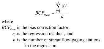
As previously discussed, bias correction factors (BCF) were used to correct the bias present in retransformed logarithmic regression equations. Duan’s (1983) smearing estimate technique was selected as an appropriate BCF to use for the flow-duration regression equations that were created using OLS regression. This BCF also has been used in other regional regression studies for OLS regression equations (Ries and Friesz, 2000; Flynn, 2003) and is computed from the following equation:
 (6)
(6)
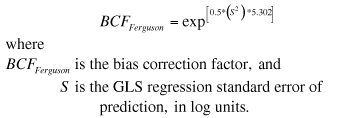
Duan’s (1983) smearing technique is not appropriate for the low-flow frequency regression equations because those equations were created using GLS regression. Because GLS regression uses a different method of computing the weighting matrix compared to OLS regression, the residuals have unequal weights (Flynn, 2003). The BCF coefficients for the low-flow frequency regression equations were computed using a technique described by Ferguson (1986) and Helsel and Hirsch (2002) as shown in the following equation:
 (7)
(7)
The computed BCF values for all flow-duration and low-flow frequency regression equations are listed in tables 7-16. The sample computations section illustrates how the BCF is used in the equations.
Final regression equations for Regions 1-10 are listed in tables 7-16, along with dependent variable constants for zero values, bias correction factors, and performance metrics. Four performance metrics were used to evaluate the adequacy of the final regression equations:
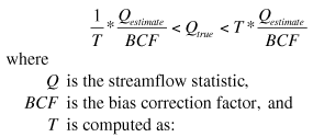
The regression equations reported here predict the values of various streamflow characteristics. The true values of those characteristics remain unknown. Prediction intervals are a measure of the uncertainty associated with the prediction made by the regression equation. The interval is the predicted value plus and minus a margin of error. The margin of error is directly related to the certainty with which the predicted value is known. A prediction interval represents the probability that the true value of the characteristic will fall within the margin of error (Hirsch and others, 1993). For example, a prediction interval at the 90-percent confidence level means there is 90-percent chance the true value of characteristic will be within the margin of error. The margin of error includes both parameter uncertainty and the unexplained variability of the dependent variables.
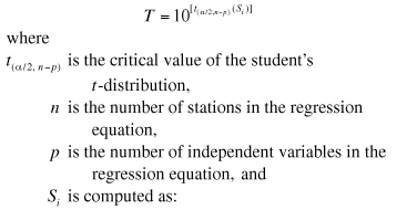
Prediction intervals are automatically calculated at the 90-percent confidence level in the StreamStats program for all 910 regression equations that were developed from this study. Equations used to compute prediction intervals and correct for bias in StreamStats are from Tasker and Driver (1988) and are shown in the following:
 (8)
(8)
 (9)
(9)
 (10)
(10)
The following is the estimate of the 50-percent flow-duration (P50) in January for Region 1 (table 7).
Assume that an ungaged stream site of interest has a basin drainage area (DA) of 200 mi2 and a mean annual precipitation (P) of 60 in/yr.
In addition to the regression coefficients (column C), this equation has a BCF adjustment of 1.01642 (column B).
P50 = 1.01642*(10-0.5732*(DA)0.9898*(P)0.7616)
P50 = 1,160 ft3/s
The following is an estimate of the 7Q2 for August in Region 7 (table 13).
Assume that an ungaged stream site of interest has a basin drainage area (DA) of 80 mi2, mean annual precipitation (P) of 20 in/yr, and a minimum slope (NS) of 0.2 degrees.
In addition to the regression coefficients (column C), this equation has a dependent variable constant adjustment value of 1 (column D). This value needs to be subtracted from the equation to compensate for a pre-log transformation adjustment that was made to the dependent variable dataset because the dataset contained one or more zero values.
The estimate is then adjusted by a BCF value of 1.46096 (column B).
7Q2 = 1.46096*[(10-4.9833*(DA)1.3556*(P)2.9361*(NS)0.4219)-1]
7Q2 = 17.9 ft3/s
In general, model accuracy tended to increase from the southeastern to northwestern regions of the study area from low-flow to high-flow conditions and from dry months to wet months. Based on equations for all 10 regions for annual and monthly flow statistics (a total of 130 values as indicated in tables 7-16), the standard errors of estimate of the high flow (5th percentile) and low flow (95th percentile) equations had medians of 42.4 and 64.4 percent, respectively. The adjusted coefficient of determination (R2adj) of the 5th and 95th percentile equations had medians of 0.95 and 0.91, respectively. A similar pattern was seen in the low-flow frequency equations. The standard errors of prediction of the equations for the 7Q2 and 7Q10 statistics had medians of 51.7 and 61.2 percent, respectively. The adjusted coefficients of determination (R2adj) of the 7Q2 and 7Q10 equations had medians of 0.94 and 0.92, respectively.
Use of the final regression equations should be limited to ungaged basins within Oregon in which the independent variables fall within the range of those sites used to develop the equations. The minimum and maximum values of all independent variables considered for each equation are shown in table 17. In addition, computations for independent variables at ungaged sites should be calculated using GIS datasets identical to those used in the study. StreamStats is populated with the same GIS datasets. If these equations are used at ungaged stream sites regulated by major reservoirs, or affected by significant diversions, they will produce estimates of natural unregulated flow conditions as opposed to actual flow conditions at those sites.
Many of the regression equations for locations in eastern Oregon are hampered by a sparser density of long-term streamflow stations, a high degree of streamflow variability, and a disproportionate amount of water use relative to streamflow. As such, careful consideration should be given to the prediction intervals when evaluating equation results for Regions 5-8, especially for low-flow equations. Depending on the level of accuracy needed, users should consider supplementing flow-statistic estimates made from the regression equations with estimates made using the drainage-area ratio, and partial-record site methods. Additional flow data collected from seepage runs along the stream upstream and downstream of the ungaged site of interest could provide an improved estimate of low-flow statistics (Riggs, 1972).
Data precision is decreased with regression equations that contain basin characteristics data created from GIS datasets. Computer generated tabular data typically are presented with arbitrary fixed decimal points. The precision of these data can not always be assumed. Final flow statistics estimated from regression equations that were created from measured flow data and GIS data should not be presented with a level of precision greater than 3 significant figures.

![]() U.S. Department of the Interior | U.S. Geological Survey
U.S. Department of the Interior | U.S. Geological Survey
URL: http://pubs.usgs.gov/sir/2008/5126
Page Contact Information: Publications Team
Page Last Modified: Thursday, 10-Jan-2013 18:52:43 EST
