Scientific Investigations Report 2008–5162
U.S. GEOLOGICAL SURVEY
Scientific Investigations Report 2008–5162
Version 1.1, December 2008
The effects of an engineered stormwater-control system on shallow ground-water flow adjacent to Lake Tahoe were simulated using a three-dimensional, finite-difference, ground-water flow model (hereafter referred to as the model). Included are descriptions of the basin-fill aquifer and quantification of components of the ground-water budget. Model results are presented as a tool to evaluate responses of ground-water flow to stormwater-runoff accumulation in the stormwater-control system. The model simulated ground-water flow and seepage across the lake interface.
Ground-water flow through the basin-fill aquifer beneath the study area was simulated using MODFLOW, a three-dimensional, numerical (finite-difference) ground-water flow model (McDonald and Harbaugh, 1988; Harbaugh and McDonald, 1996). The model area was discretized into a grid of 23,925 rectangular model cells in 165 rows and 145 columns areally and 6 layers vertically. Each model cell was about 66 ft wide in the row and column dimensions and had variable thickness. The model grid was rotated 25 degrees clockwise about row 83 and column 73 (UTM NAD 1983, zone 10N 763,855.52, 4,316,204.58 meters) so that the major axes were parallel to the general direction of ground-water flow, which generally is toward the lake in the model domain. Rotation of the grid caused 43 percent of the cells to fall outside the area of interest; therefore these cells were inactive. The top of layer 1 represented land surface and covered about 2.1 mi2. The southeast boundary extended upgradient to where bedrock is quite shallow, generally along the 6,350-ft topographic line. A sharp dropoff of the lake bottom served as the submerged northwest boundary (fig. 5).
Aquifer thickness generally is very thin near the upgradient southeast boundary and thickens toward and under the lake (fig. 6). Total aquifer thickness along the upgradient boundary mostly is less than 50 ft, while along the northwest boundary beneath Lake Tahoe, it is nearly 1,500 ft thick (Eric LaBolle, University of California, Davis, written commun., 2006).
The model objective was to understand movement of shallow ground water; therefore a finer discretization was used in the upper 50 ft of the model domain (fig. 6). Model layer thicknesses in layers 1–5 were designed to keep uniform thickness throughout each individual layer. Layer 1 was a constant 5 ft thick, while layer 2 was a constant 10 ft thick. Layers 3–5 were each a constant 15, 10, and 10 ft thick, respectively. Layer 6 varies in thickness from the bottom of layer 5 to bedrock. The large and varying thickness of layer 6 is assumed to have no effect on the simulation of shallow ground-water movement, although it likely stores a large quantity of ground water. Discontinuous lacustrine units typically are less than 20 ft in thickness and likely are reworked by meandering streams; therefore a continuous confining unit was not simulated in this model.
Shallow ground-water flow was simulated as a steady-state flow system. Annual Lake Tahoe stage fluctuations will have a time-varying effect on nutrient loads discharged by ground water, although in evaluating the suitability of a detention basin as a BMP, long term loading is more of a concern. Therefore, modeling the transient ground-water system as a steady-state flow system is considered sufficient for the model objectives.
Various boundary conditions were used across the model (fig. 5). All interior model cells exposed to Lake Tahoe in the northwest were simulated using a constant-head boundary of 6,225 ft, which is the average stage of Lake Tahoe over the study period. The southern Park Avenue detention basin (PA1), which contained standing water throughout the study, also was simulated using a constant-head boundary in six contiguous cells. A network of stormwater drainage ditches and sewers scattered across South Lake Tahoe were simulated using drains (Jim Marino, city of South Lake Tahoe, written commun., 2006). These drains were placed 5 ft below land surface. In this way, if the simulated ground-water surface came within 5 ft of land surface, ground water would discharge to the stormwater ditches and flow directly to Lake Tahoe.
Recharge was applied to the onshore modeled area by areal recharge and mountain-front recharge from watersheds upgradient of the study area. Areal recharge, for the purposes of this model, was defined as precipitation that passes beneath the root zone and crosses the water table. All layer 1 onshore pervious model cells or those cells simulated as not being impervious due to urbanization (about 62 percent of all active layer 1 cells; Raumann, 2007) received areal recharge. The volume of areal recharge was estimated during model calibration and constrained by local precipitation and evapotranspiration estimates.
Mountain-front recharge was defined as surface runoff from contributing watersheds that flows over bedrock and infiltrates at the bedrock-alluvium contact. Mountain-front recharge was applied to all cells along the southeast domain boundary, as well as to two adjacent zones that extend northwest from the mountain front (fig. 5). The two larger zones represent small drainages where coarser grained material is present (Rogers, 1974); therefore, mountain-front recharge naturally is greater in these locations (fig. 7). The volume of annual precipitation averaged 4,400 acre-ft in the watersheds upgradient of the model area between 1971 and 2000 (Flint and Flint, 2007). Results from Flint and Flint indicated that of the total precipitation about 2 percent becomes in-place recharge, 54 percent is consumed by evapotranspiration, and the remaining 44 percent is attributed to potential runoff. The percentage of the potential runoff that actually becomes mountain-front recharge was estimated during model calibration.
No-flow boundary conditions were used in several locations in the model (fig. 5). Bedrock underlies all of layer 6 and represents a no-flow boundary. Model boundaries to the northeast and southwest were aligned along hydrologic basin boundaries (Cartier and others, 1995) and therefore were represented as no-flow boundaries.
Calibration is the attempt to reduce the difference between model results and measured data by adjusting model parameters. The improvement of the calibration is based on minimizing the differences between simulated and measured ground-water levels. The discrepancy between model results and measurements (known as the residual) commonly is, in part, the cumulative result of simplification of the natural system by the conceptual model, the model grid, and the scarcity of sufficient data to account for the spatial variation in hydraulic properties and recharge throughout the study area.
Uniform hydraulic conductivity distributions were assigned throughout all model layers because of limited hydraulic information. Calibration was constrained by assuming the transmissivity of the alluvial aquifer was known from a pump test completed in wells near the Park Avenue detention basins. Transmissivity is equal to the hydraulic conductivity of aquifer materials, multiplied by the aquifer thickness. The pump test completed by the South Tahoe Public Utility District yielded transmissivity estimates of 1,800 ft²/d (fig. 5; Bergsohn, 2000). Horizontal hydraulic conductivity was 2 ft/d and was not estimated during model calibration. This resulted in a transmissivity estimate of 2,000 ft2/d near the Lake Tahoe shoreline, where the aquifer has a thickness of about 1,000 ft (fig. 6). This is reasonable as it falls into the 0.3–20 ft/d range of values (median value of 3 ft/d) estimated from slug tests (table 2). Discontinuous lacustrine units were assumed to be distributed uniformly throughout the aquifer and were simulated in the average vertical hydraulic conductivity. Vertical hydraulic conductivity was assumed to be lower in the six cells between layers 1 and 2 beneath PA1 because of sediment compaction during basin construction. Vertical hydraulic conductivities were estimated during model calibration.
The ground-water flow model was calibrated to average water-level measurements in 18 wells. The following weighted (w)i, sum-of-squares (SS) objective function was minimized during calibration,
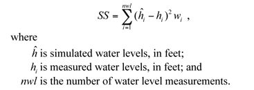 (1)
(1)
Note: The root-mean-square (RMS) error is reported instead because RMS error is more directly comparable to actual values and serves as a composite of the average and the standard deviation of a set. RMS error is related to SS error by
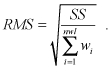 (2)
(2)
Model calibration was further facilitated by parameter estimation. Estimated parameters included (1) the volume of potential runoff generated in the watersheds adjacent to the modeled area that becomes mountain-front recharge along the southeast boundary, (2) the volume of areal recharge distributed homogeneously to pervious model cells, (3) the vertical hydraulic conductivity in the area surrounding the Park Avenue detention basins, (4) the vertical hydraulic conductivity of the remaining aquifer, and (5) stormdrain conductance.
Each parameter was changed a small amount and MODFLOW was used to compute new water levels for each perturbed parameter. As a secondary calibration procedure, recharge rates were bracketed within 200 and 450 acre-ft/yr (Flint and Flint, 2007). Vertical hydraulic conductivity near Park Avenue detention basins, also was given an upper limit lower than that of estimates at Cattlemans detention basin of 0.027 ft/d because PA1 remains wet year round, whereas Cattlemans is dry for many months per year (Green, 2006). An iterative process was followed by estimating parameters, running revised models using the estimated parameters, and calculating new water levels until the objective function change was minimize and could not be improved.
The final calibrated model was the best fit possible of the observed water levels given the parameter constraints described above. Simulated water levels representative of conditions from 2005 to 2007 approximated the 18 measured water levels in the modeled area (fig. 8). Fourteen shallow wells were screened within layers 1 and 2 (within 15 ft below the water table) and 4 deep wells were screened within layer 3 (between 15 and 30 ft below the water table). However, simulated water levels did not exactly reproduce all measured water levels in all wells. Figure 9 shows the simulated water-level contours and monitoring well residuals. Measured water levels in a cluster of wells within about 300 ft of each other in the south-central part of the model (wells B-3, B-4, Beach, and Azure) ranged about 1.5 ft. The flow model assumes homogeneous aquifer properties and therefore was not able to simulate such a span of water levels in close proximity to each other. Simulated water levels near model boundaries may be less reliable than simulated water levels that are distant from boundaries. Boundary effects are most notable when there are nearby stresses. For instance, detention basin PA1 was simulated with a constant-head boundary of 6,234 ft. Observed water levels in wells upgradient and downgradient of PA1, however, were 4–5 ft lower than this level. Therefore, the model was not able to simulate accurately such a localized field condition. During the construction of PA1, sediment possibly was compacted in the basin, resulting in stormwater inflow being semiperched above the regional water table. Small drains discharging water in the south-central part of the model near wells B-1 and NWIS5601 also affected the accurate calibration of water-level contours. Average measured water levels in these wells differed by 10.5 ft, and therefore had rather large simulated residuals. The final calibrated model produced a RMS error of 2.55 ft.
The final calibrated values for model parameters are listed in table 5, and components of the water budget are shown in figure 10. Total mountain-front recharge was estimated as 306 acre-ft/yr. This value is comprised of 2 percent of precipitation as in-place recharge as computed by the Basin Characterization Model of Flint and Flint (2007) and a calibrated value of 16 percent of runoff becoming recharge. These values are within the bounds present by Flint and Flint (2007). Areal recharge was estimated quite low at about 5 acre-ft/yr and recharge from detention basin PA1 was about 1 acre-ft/yr. Drains used to simulate storm ditches were estimated to discharge about 56 acre-ft/yr, allowing ground water to exit the subsurface and discharge to the lake. Direct ground water discharge from the study area to Lake Tahoe was 256 acre-ft/yr. About 75 percent of ground-water discharge to Lake Tahoe occurs from layer 1. The distribution is shown in figure 10.
To determine how model parameters affected simulation results, all estimated parameters were varied independently from 0.2 to 5 times their calibrated value. This range was greater than the uncertainties associated with the parameters, but provided a more complete perspective on model sensitivity. Model sensitivity was described in terms of the RMS error. The sensitivity of model results to changing one parameter while all others are held at their calibrated values is shown in figure 11. Residuals were determined to be more sensitive to changes in mountain-front recharge, especially through the course-grained channel to the northeast than to any other model parameters. Model results were rather insensitive to storm-drain conductance and vertical hydraulic conductivity of the detention basin and the rest of the model.
Model sensitivity to specified boundary conditions and hydraulic properties was further investigated with four alternative models. Alternative models included increasing the stage of Lake Tahoe within the constant-head boundary to 6,229 ft (historical high watermark), lowering it to 6,223 ft (altitude of lake outlet at Tahoe City Dam), incorporating a clay layer into the hydrogeology, and increasing the model horizontal hydraulic conductivity from 2 to 4 ft/d. The continuous clay layer was simulated in the model by reducing the horizontal hydraulic conductivity of only layer 3 to 0.001 ft/d. Each alternative model was calibrated after changing the selected boundary conditions and hydraulic properties. Results of these alternative models are listed in table 5.
Computed RMS error of the four alternative models varied by about 1.4 ft. Raising the stage of Lake Tahoe had the greatest effect on the model error by reducing it by about 1.2 ft. As expected, discharge to Lake Tahoe was reduced when the stage of Lake Tahoe was increased because it has a direct effect on the hydraulic gradient within the model. In response to a shallower gradient, the mountain-front recharge was decreased within the calibration process to allow ground-water levels in the aquifer to approach their observed elevations. Model error was insensitive to simulations of (1) lowering the stage of Lake Tahoe, (2) layer 3 representing a continuous clay layer, and (3) increasing the horizontal hydraulic conductivity to 4 ft/d.
The flow model reasonably describes local ground-water flow near the Park Avenue detention basins, but it cannot mimic exactly the true ground-water flow system. Simulated values often are similar to, but do not match precisely with the measured values. The ground-water flow model is a numerical approximation of the flow system, and is limited by simplifications in the conceptual model, discretization effects, and the scarcity of measurements to account for the spatial variation in hydraulic properties throughout the study area.
Inherent in the conceptual model is the assumption that all sources of flow and stresses on the natural system are represented in the numerical model. Because measurements of water levels used to constrain the model calibration were made over a short time period, it is not known how completely or how accurately the numerical model simulates the natural system, especially under steady-state conditions.
Areal discretization of the study area into a rectangular grid of cells and vertical discretization into layers required averaging of hydraulic properties. Each model cell represents an averaged block of the aquifer system. Due to this averaging, the model cannot simulate the local effects on flow caused by aquifer heterogeneity. Further simplification of the heterogeneous aquifer system occurred in the methods used to describe the distribution of the hydraulic conductivity. The lack of sufficient measurements to account for the spatial variations in hydraulic properties necessitated the uniform assignment of horizontal hydraulic conductivity across the study area. Simplifying the model to this degree does not invalidate the model results, but should be considered when interpreting the results.
The reliability of ground-water flow models is affected by the choice and accurate representation of the aquifer and related boundary conditions. For purposes of simplification, the upper model boundary (land surface) was simulated as a confined system. The variations in transmissivity with respect to water-level change were trivial and limited error was introduced as a result of this simplification. A one-to-one correlation does exist between uncertainties of assigning transmissivity and estimating recharge. For example, a lower hydraulic conductivity, which yields a lower transmissivity, does not require as much water for simulated heads to approach measured heads. In turn, a lower recharge is estimated. Measured water levels in a well cluster in the southern part of the model varied about 2.9 ft; therefore the model, assuming homogeneous aquifer properties, was not able to accommodate such a span of water levels in close proximity to each other. Simulated water levels near model boundaries may be less reliable than simulated water levels that are distant from boundaries. Boundary effects are most notable when there are nearby stresses. For instance, PA1 was simulated with a constant-head boundary of 6,234 ft and observed water levels, upgradient and downgradient, were 4–5 ft below that of PA1. Therefore, the model was not able to simulate such a localized field condition. During the construction of PA1, sediments possibly were compacted and resulted in stormwater inflow being semiperched on a less conductive area of aquifer.

![]() U.S. Department of the Interior | U.S. Geological Survey
U.S. Department of the Interior | U.S. Geological Survey
URL: http://pubs.usgs.gov/sir/2008/5162
Page Contact Information: Publications Team
Page Last Modified: Thursday, 10-Jan-2013 18:56:41 EST
