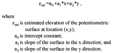
Methods of Investigation

Methods used to compile and analyze information to characterize shallow groundwater movement in the study area include measurement of water levels in wells, estimates of Skagit River stage, construction of water-level maps, and determination of ocean tides.

Well Inventory and Water-Level Measurements

Characterization of the groundwater-flow system relied on the analysis of spatially distributed information about groundwater levels, and the physical and hydraulic properties of the geologic units detected during well construction. This information was obtained through the measurement of water levels in wells, and the evaluation of lithologic descriptions from well drillers’ logs. Lithologic information was used to identify wells completed in the shallow groundwater system. Well records were compiled from USGS and Washington State Department of Ecology databases to identify potential wells to be used in this study. Candidate wells were selected for field inventory based on the location and depth of the well, and the availability of the drillers’ log. The goal of the inventory was to obtain an even distribution of wells throughout the study area. However, this was not possible for the entire study area because of a lack of wells in less populated areas. During the field inventory in August 2007, permission was obtained to measure water levels in 43 wells (fig. 3) on a quarterly basis (August 2007, November 2007, February 2008, and May 2008). Four additional wells were added to the quarterly monitoring network as they became available for measurement. One of these wells (34N/03E‑35N01) was installed for this study using a rotary drill rig and constructed of 6 in. steel casing and 0.01 in. stainless steel screen. Four quarterly monitoring wells were instrumented with continuous water-level recorders (fig. 3).

The depth to groundwater below land surface was measured using a calibrated electric tape or graduated steel tape, both with accuracy to 0.01 ft. Latitude and longitude locations were determined for each well using a Global Positioning System receiver with a horizontal accuracy of one-tenth of a second (about 10 ft). Altitudes of the land surface at each well were interpolated from USGS 1:24,000–scale topographic maps, with an accuracy ranging from ±5 ft (low-relief areas) to ±10 ft (high-relief areas). Light Detection and Ranging (LiDAR) derived values for the altitude of land surface became available after completion of the field inventory, and were used to determine the altitude of land surface at each well for the computation of water-level altitudes. LiDAR data were collected and processed by a private vendor under contract with the USGS. Vertical accuracy was evaluated for internal consistency (repeatability), and conformance with independent ground-control points.

All water-level measurements were made by USGS personnel according to standardized techniques of the USGS (Drost, 2005). Well information collected during the field inventory and the quarterly monitoring-network measurement periods were entered into the USGS National Water Information System (NWIS) database and published in Fasser and Julich (2009).

River Stage

Estimates of Skagit River stage (the altitude of the water surface in the river) were used to constrain groundwater-level contours along the eastern margin of the study area, and to infer groundwater recharge from or groundwater discharge to the river. Daily values of river stage were obtained for USGS steamflow-gaging station 12200500 (Skagit River near Mount Vernon, Wash.; fig. 3) and a mean gage height was computed for each of the quarterly monitoring-network measurement periods. The initial measurement period (August 2007) required locating suitable wells and obtaining owner permission and took 8 days to complete. All subsequent quarterly measurements (November 2007, February 2008, and May 2008) were accomplished in 2 days. Values of river stage reported in vertical datum NGVD 29 were converted to the datum used for the monitoring network, NAVD 88, using the on-line program VERTCON (http://www.ngs.noaa.gov/cgi-bin/VERTCON/vert_con.prl) provided by the National Geodetic Survey.

River stage at the USGS steamflow-gaging station was extrapolated along the length of the Skagit River within the study area using several data coverages and Geographic Information System (GIS) procedures. Spatial data points were developed to represent the centerline of the river based on available coverages of hydrography, aerial photography, USGS quadrangle topographic maps, and LiDAR imagery. These data were cross checked, and adjusted using ArcMap^TM, version 9.3, by ESRI Inc., to produce a consistent rendering of river hydrography. The points for the centerline were converted to x and y coordinates (NAD 83 State Plane Washington North) in the software, and exported to Microsoft Excel^®. The distances between centerline points were computed and summed to obtain a total distance from the mouth of the Skagit River. River channel distance was measured along the North Fork of the Skagit River, and extended out of the study area to open water in Skagit Bay, where water levels were expected to average to mean sea level. The total river mile distance from open water to the USGS gage was computed to be 17.5 mi. GIS points were then interpolated at one-half-river-mile intervals, and each point was assigned a river-stage value by proportionally adjusting the stage value at the USGS gage (for example, by a factor of (river mile)/17.5).

These estimates of river stage were considered during construction of groundwater-level maps and were compared to nearby groundwater levels measured in the delta to help infer the nature of the hydraulic connection between the Skagit River and adjacent groundwater system. In areas where estimates of river stage were higher than nearby groundwater levels, the potential for groundwater recharge from the river exists, and the orientation of groundwater-level contours were drawn to reflect surface-water recharge.

The linear interpolation described above might differ from the actual stream-stage values due to unaccounted for variations in river hydraulics such as changes in cross section, gradient, and the effects of distributary channels (such as the South Fork of the Skagit River), and tidal influence. To check the procedure, LiDAR altitudes were obtained with GIS at the points used for estimating river miles. Despite the fact that the laser is reflected and/or absorbed rather than directed back to the detector, it seems that sufficient LiDAR elevation points are picked up immediately along the banks of the river to give a good estimate of river stage along the river. Linear regression of the LiDAR data indicated a linear relation between river mile and LIDAR derived river stage of 0.99 ft/mi, corresponding to a river stage value of approximately 16.5 ft at the USGS gaging station. The computed mean gage height at the USGS gaging station for the quarterly measurement periods ranged from 16.46 to 25.63 ft. The regression analysis of LiDAR data gave a good fit to the linear interpolation of river stage with a root-mean-square error of 1.75 ft for the data points available, and supports the use of linear interpolation to estimate river stage.

Groundwater-Level and Flow-Direction Maps

Of the 47 wells inventoried (fig. 3), measurements from 34 wells completed in alluvial deposits (shallow groundwater system) were used in the construction of groundwater-level and flow-direction maps, and linear-regression analysis. Groundwater level (altitude) was calculated by subtracting depth to water from the LiDAR derived ground-surface altitude at each well. Groundwater-level altitude contours and flow lines were generated manually for each of the quarterly measurement periods. Wells completed in glacial deposits or below confining clay layers within the alluvium were not included in the construction of groundwater-level and flow-direction maps or linear-regression analysis because water levels from these wells are likely influenced by hydrogeologic conditions that are distinctly different from those controlling water levels in the shallow groundwater system. Furthermore, upland areas consisting of relatively low permeability glacial deposits and bedrock were interpreted as probable shallow groundwater-flow barriers.

Water levels in well 22F02 were influenced by active pumping during all quarterly measurements, and water levels in well 26Q01 were significantly lower than surrounding wells leading to uncertainties regarding the accuracy of well-construction and lithologic information or the possibility of nearby pumping. Therefore, water-level data from these two wells were not used in the construction of groundwater-level and flow-direction maps or linear-regression analysis. Water levels in wells 08R01 and 20J01 were influenced by pumping during the August 2007 quarterly measurement and were not used for the construction of maps or regression analysis. Some wells only had partial water-level records (water levels were not available for all quarterly measurements) and were only used in the construction of maps and regression analysis for quarterly measurements in which data were available. Hydrographs of groundwater levels were generated for all inventoried wells and published in Fasser and Julich (2009).

A linear-regression analysis of groundwater altitudes in the Skagit Delta area was done to estimate the overall, time-averaged shallow groundwater-flow direction and gradient. The data used in the regression analysis were similar to those used for construction of the groundwater-altitude maps and included: (1) x and y coordinates for the wells according to the NAD 83 State Plane projection in feet for Washington (North) and (2) quarterly groundwater altitudes from the 34 wells completed in alluvial deposits.

The regression analysis was calculated using Microsoft Excel^® Data Analysis tool. Each set of quarterly water-level measurements was analyzed separately, and then the seasonal regression coefficients were combined to obtain an overall (annual) flow regime description. The groundwater altitudes (z) were input as the dependent variable and the two columns of x and y coordinates of the wells were entered as the independent variables. In this case, linear regression was used to estimate coefficients a₀, a₁, and a₂ that describe a planar surface for the potentiometric surface as:

     (1)

These coefficients were then used to estimate the common hydrogeologic parameters of the groundwater regime for that quarterly measurement:

Gradient = SQRT (a₁² + a₂²) is the slope of the potentiometric surface.

Direction = ATAN2 (a₁, a₂) is the upstream/downstream direction of the surface.

Then, the relative water level was calculated as the elevation of the plane at the geographic center of all well locations (centroid; fig. 3):

Water level at the centroid = z _cent = a₀ + a₁ * x _cent + a₂ * y _cent

After measurements for all four sets of quarterly measurements were processed through the regression method, an estimate of direction and gradient of the annual groundwater system was calculated by averaging the regression coefficients from each of the quarterly measurements, for example:

a_{0, annual} = (a_{0, August} + a_{0, November} + a_{0, February} + a_{0, May}) / 4

After averaging to get the annual coefficients, the annual gradient, direction, and water level at the centroid were calculated from the annual regression coefficients.

Ocean Tides

Predicted values of tidal extremes were used in an analysis of possible correlation between groundwater-level fluctuation at monitoring well 19F01 (fig. 3) and ocean tides. The tide data were obtained from the closest National Oceanic and Atmospheric Administration tide gage (National Oceanic and Atmospheric Administration, 2009) that had calibrated tidal coefficients (tide gage 9448558 “La Conner, Swinomish Slough, Wash.”). The resulting analysis (discussed later in this report) is only approximate, because of several factors: (1) the groundwater-level data from well 19F01 also were influenced by recharge or other factors; (2) the tidal record used in the analysis is only of predicted astronomical highs and lows, not actual measured tidal levels, that may have been affected by wind and barometric pressure; (3) the location for the predicted tide is at La Conner, more than 2 mi to the south, not at the point in Swinomish Channel closest to the well, and different tidal components may travel differently along the narrow and shallow channel; and (4) high tides seem to have less influence on the well than do low tides (estimated from the correlation coefficients), although this may be caused by tidal attenuation along the Swinomish Channel.