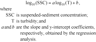
Methods and Data Analysis

Data Collection

Eight water-quality monitoring stations were in operation in the North Santiam River basin during water year 2008. Streamflow data were collected at seven of these monitoring stations. (The City of Salem’s water treatment facility intake, located at Geren Island, is monitored for water quality only.) All preliminary data are available in near real-time on the project website (U.S. Geological Survey, 2009a). Published data are available through the USGS National Water Information System (NWIS) website (U.S. Geological Survey, 2009b).

Station Instrumentation

Water-quality data were collected in accordance with the maintenance and calibration protocols described by Wagner and others (2006) for water temperature, specific conductance, pH, turbidity, and dissolved oxygen (table 2). All water‑quality monitoring stations were equipped with a YSI 6920 multi-parameter instrument. Turbidity was measured by a YSI 6026 sensor in Formazin Nephelometric Units (FNU) (Anderson, 2005). Each of these sensors has a different maximum turbidity value, ranging from 1,200 to 1,800 FNU. All parameters were recorded at 30-minute intervals by a data‑logger and uploaded every 3 to 4 hours to the USGS database.

Suspended-Sediment Sampling

Suspended-sediment samples collected at the monitoring stations provided the data necessary to relate the optical property of turbidity to the concentration of sediment in the river. Suspended-sediment samples were collected at each monitoring station using standard USGS methods (Edwards and Glysson, 1999). All samples were analyzed for suspended‑sediment concentration (SSC) in milligrams per liter. In addition, many samples were analyzed for percent of silt and clay and reported in percent finer than 62 µm in diameter.

The equal-width-increment (EWI) method was used to collect most cross-sectional, depth-integrated samples (Edwards and Glysson, 1999). Automatic pumping samplers were installed at the three stations in the upper basin. These samplers were programmed to collect single-point samples from a location near the in-situ water-quality instrument when the instream turbidity reached a specific threshold value (usually 20, 50, or 100 FNU). Point samples were collected at regular intervals until the turbidity was less than that same threshold value.

Quality Assurance

Cross-Sectional Samples

During the period of the North Santiam River basin study (water years 1999–2008), more than 100 replicate cross‑sectional samples were collected at the seven stations to assess the precision of the sampling methods and of the laboratory results. An ordinary least-squares linear regression analysis was completed between the SSC values of pairs of concurrent samples (fig. 3). The result was a highly correlative (R² = 0.98) and close to 1:1 relation (slope = 1.07) over a wide range of SSC values (1–400 mg/L).

Point Samples

The automatic samplers at the three upper-basin stations were activated regularly before and after collection of EWI samples to assess the representativeness of single‑point SSC to cross-sectional SSC. The SSC values of each pair of point samples were interpolated to the mean time of the corresponding EWI sample. An ordinary least-squares linear regression analysis was performed on the data from each monitoring station (table 3). The results show good correlation between the automatic point samples and the cross‑sectional EWI samples at North Santiam and Breitenbush over the entire range of sample SSC values (10–14,500 and 2–660 mg/L, respectively). Results from Blowout also show good correlation, except at high SSC (greater than 400 mg/L) and high streamflow (greater than 2,500 ft³/s). As a result, any point samples collected at Blowout when either of these conditions was exceeded were not included in further data analysis.

Serial Correlation

The point samples at the three upper-basin stations were shown to be acceptably representative of their respective cross sections, but the large number of these samples and the timing of their collection likely would introduce serial correlation biases into the regression analyses. The vast majority of the more than 550 point samples collected by the automatic samplers during water years 2004–08 were caused by high‑turbidity conditions. Once an automatic sampler was activated, samples were collected until the instream turbidity was less than the threshold value. As a result, as many as 24 samples could be collected during a single storm. In order to minimize the potential bias, one to three point samples (depending on the duration of the event) were selected randomly from any single storm or sampling event for inclusion in the model calibration datasets.

Data Analysis

Regression models were developed between sample suspended-sediment concentration (SSC) and turbidity (T) as a means of estimating continuous SSC using continuous turbidity data. The estimated SSC and streamflow (Q) were then used to compute annual suspended-sediment loads (SSL) at each of the monitoring stations for water years 2005–08. Uhrich and Bragg (2003) and Bragg and others (2007) previously reported the methods for this analysis.

Regression Models

Regression models were developed between turbidity and SSC for each of the monitoring stations. Turbidity data for the analyses were provided by the instream water-quality monitors. The 30-minute turbidity values, in FNU, recorded during the time of sample collection were averaged to produce a single turbidity value associated with each sample. The SSC values, in milligrams per liter, were provided by laboratory analysis of each sample (Guy, 1969). The pairs of turbidity and SSC data for each sample were used as the calibration dataset for the regression model.

The turbidity and SSC values were transformed to base‑10 logarithmic values to improve the normal distribution of the dataset prior to ordinary least-squares linear regression analysis. The form of the regression model equation is:

(1)

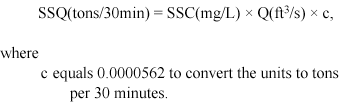
The logarithmic transformation and subsequent conversion back to original form introduced a known bias, which was negated with a correction factor (Helsel and Hirsch, 2002). The predicted SSC value resulting from the model equation was multiplied by the bias-correction factor to obtain the corrected SSC value (table 4).

North Santiam Regression Models

The operation of the automatic sampler at the NorthSantiam station revealed a process of sediment transport that had not been addressed in previous analyses. Two instances of high turbidity (greater than the turbidity sensor limit of about 1,600 FNU) with no corresponding increase in streamflow were investigated by Sobieszczyk and others (2007). The sediment causing the high turbidity was associated with meltwater from the glaciers and snowfields in the Milk Creek and Pamelia Creek subbasins, located high on the slopes of Mount Jefferson (fig. 1). Analysis of the samples collected during these events revealed a relation between instream turbidity and SSC that was different from that normally measured during typical storm events, necessitating the revision of the previously published regression model (Bragg and others, 2007).

The previous model included samples collected at NorthSantiam during water years 1999–2004. For the revised analysis, all suspended-sediment samples collected during those years were categorized on the basis of the conditions during which they were collected. Typically occurring in late summer or early fall, glacial outwash events resulted when warm air temperatures rapidly melted glacial ice and snowfields, transporting newly exposed sediment downstream. These events were identified at the monitoring station by a sharp increase in turbidity but little or no increase in streamflow. The summer melting of snow and ice at high elevations also caused small-magnitude diurnal cycles of streamflow and turbidity at North Santiam. Samples collected during either of these conditions were classified as “meltwater‑driven.” During the fall and winter rainy season, increases in instream turbidity usually were accompanied by a proportional increase in streamflow. Samples collected during these conditions were classified as “precipitation-driven.” The two newly classified sample sets were used to develop two new regressions to replace the single previous regression (fig. 4). The new regression models were not used to revise previous suspended-sediment load computations, but only to establish benchmark models for future analysis. Both revised North Santiam regression models were updated for each subsequent water year as described below.

Updated Regression Models

As water-quality data collection continued at all monitoring stations, the regression models required updating and verification. The regression models reported in Bragg and others (2007) were developed with suspended-sediment samples collected through water year 2004. Beginning in water year 2005, a newly established method for annually updating the regression models involved adding samples collected during each subsequent water year to the model calibration dataset (Rasmussen and others, 2009). The regression analysis at each monitoring station was repeated with the complete dataset to determine whether the coefficients (a and b, eq. 1) of the new equation had changed significantly from the equation used the previous water year. If no significant difference was detected between the two model equations, the regression model incorporating the newly collected samples was used to calculate the continuous SSC record for that water year. If the coefficients were significantly different, a new regression model could be established with either the samples collected after the date of a known change in sediment source or the samples collected during the new water year. The water year 2008 regression models (table 4) include samples collected during the entire period of suspended-sediment sampling for each station (table 2). A table of annually updated regression models for all stations for all water years (1999–2008) is available in appendix A.

The North Santiam regression models for precipitation‑driven events demonstrated a significant 
change from water year 2006 to 2007 (appendix A). An analysis of the covariance between the two models indicated 
a significant difference in the slope (a; which increased) and the y-intercept (b; which decreased). This shift likely was a result of the inclusion of samples collected in the days and weeks following the November 2006 debris flow on Mount Jefferson. These samples reflected the documented change in available sediment in the upper elevations of the basin, which persisted through the water year. The water year 2007 model that incorporated the new samples was therefore used to calculate the precipitation-driven portions of the continuous SSC record for North Santiam. The water year 2008 precipitation-driven model shifted slightly in the opposite direction (the slope decreased and the y-intercept increased), indicating that the effect of the additional sediment source may have been largely temporary.

Error Analysis

Several of the summary statistics recommended by Rasmussen and others (2009) were computed to evaluate the regression models (table 4). The coefficient of determination (R²) indicates the part of the variance explained by the regression. The root mean squared error (RMSE) of the regression was calculated in log-10 units and converted to the upper and lower model standard percent errors (MSPE). These percentages indicate the variance between the predicted and measured values and can be used to compare regression models. For example, lower magnitude MSPE values indicate less uncertainty in the predicted values. These statistics were considered when evaluating SSL computations and comparing SSL values between monitoring stations.

Regression models for water year 2008 for stations in the upper North Santiam River basin indicated high R² values and acceptable MSPE values. The regression models for the two lower-basin stations subject to streamflow regulation by the dams showed the most uncertainty. The R² value was lower at Niagara, but the MSPE range was comparable to the upper‑basin stations. The MSPE range was greatest at Mehama, indicating the highest uncertainty in predicted SSC values. The greater uncertainty was attributed to the varied turbidity bias in the cross-section at Mehama resulting from the regulated streamflow from Big Cliff Dam and from the confluence of the Little North Santiam River less than 1 mile upstream of the station.

Estimation of Missing or Erroneous Values

Missing Turbidity Values

A complete SSC record, in 30-minute time increments, was needed to compute annual SSL. When turbidity values used to calculate SSC were missing from the record, values were estimated by several methods. Using the simplest method, the 30-minute values were estimated by interpolating between the recorded values immediately before and after the missing period. This method worked well for short time periods when streamflow conditions were steady or when turbidity consistently was increasing or decreasing. For longer periods or during changing streamflow conditions, turbidity was estimated by comparing values at adjacent monitoring stations. This method worked best when two stations had long periods of record that demonstrated a well-defined correlation between turbidity values.

The turbidity at Rock was estimated for several periods of missing or erroneous data. Correlation with Little North data was used to complete the turbidity record for December 15, 2006–January 5, 2007, which included a moderate storm event. Interpolation was used to complete the Rock turbidity record during the low-streamflow periods of January 26–March 5, 2008, and May 18–27, 2008. The other stations in the monitoring network had few instances of missing 30-minute turbidity values and were estimated by simple interpolation. The estimated turbidity values were used to calculate SSC at each respective monitoring station.

North Santiam Suspended-Sediment Concentration

During one major sediment transport event, the continuous SSC record was computed more directly from samples, rather than from estimated turbidity. The debris flow that occurred in the Pamelia and Milk Creek subbasin on Mount Jefferson resulted in extremely elevated turbidity and SSC at North Santiam on November 6–7, 2006. When the recorded turbidity values remained constant at 1,600 FNU on November 6 during 0200–0730 and 0930–1600, the instream turbidity was known to be equal to or greater than that value. During these periods, more than a dozen point and EWI samples were collected (fig. 5). On November 6 during 0800–0900, several turbidity values were recorded that were less than the sensor maximum value. The meltwater-driven regression model was used to estimate SSC during these times because no samples were collected. Using a combination of sample SSC, turbidity-estimated SSC, and interpolation, the continuous SSC record was completed for this unusual event. The estimated 30-minute SSC computations for North Santiam on November 6–7, 2006, are available in appendix B.

Computations of Suspended-Sediment Load

Estimated 30-minute SSC (in mg/L) and corresponding streamflow (Q) values, in cubic feet per second (ft³/s), were used to calculate the suspended-sediment discharge (SSQ; equation 2), in tons per 30 minutes:

(2)

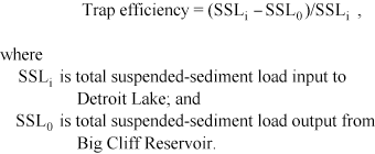
The daily SSL is computed by summing the 48 estimated SSQ values per day. The annual SSL is calculated by summing the 365 (or 366) daily SSL values.

Prediction intervals were calculated for each of the regression models in order to provide error estimates for the annual SSL values. For each estimated 30-minute SSC value, the upper and lower predictions were calculated at 90 percent confidence. High and low annual SSL totals were calculated as described above from the continuous upper and lower SSC prediction records.

Computations of Suspended-Sediment Budget

Annual SSL totals were used to summarize the suspended-sediment budget in the North Santiam River basin for water years 2005–08 (fig. 6). The SSL from the three stations in the upper basin (North Santiam, Breitenbush, and Blowout) were summed to compute the sediment input to Detroit Lake. The SSL at Niagara represented the sediment output from Detroit Lake and Big Cliff Reservoir. The total SSL flowing past Geren Island was defined as the sum of Niagara, Rock (if data were available), and Little North. Although the SSL was estimated at Mehama for all water years, it was not used in the sediment budget because of the high uncertainty of the regression models.

The relative percent contribution of each monitoring station to each step of the suspended-sediment budget was computed for each water year. In addition, the relative percent contribution of each monitoring station was computed for the total 4-year suspended-sediment budget of water years 2005–08.

The total suspended-sediment budget for water years 2005–08 also was analyzed by month to examine and quantify the season for peak sediment transport. The monthly sums for each step of the budget (input to Detroit Lake, output from Big Cliff Reservoir, and flow past Geren Island) were expressed as a percentage of the total 4-year sediment budget.

The difference between the sediment input to Detroit Lake and the sediment output from Big Cliff Reservoir (as measured at Niagara) was used to estimate the combined trap efficiency of the reservoirs (eq. 3).

(3)

About 27 percent of the water volume measured at Niagara during water years 2005–08 was not accounted for by the streamflow measured at the three upper-basin monitoring stations. Reservoir storage changes, groundwater input, and unmonitored tributaries could account for the water volume difference. Because the trap efficiency calculation did not account for the sediment input associated with any unmeasured streamflow entering Detroit Lake, there likely was a negative bias on the estimates. The actual annual trap efficiencies of Detroit Lake and Big Cliff Reservoir likely were higher than the calculated values.

Historic Streamflow

Streamflow data from two of the monitoring stations in the North Santiam River basin were analyzed to provide context for the suspended-sediment load and budget computations. Annual streamflow is highest at North Santiam in the upper basin and, for unregulated streams, at Little North in the lower basin. Annual mean streamflow for water years during the period of the North Santiam River study (water years 1999–2008) are shown in figure 7. The median value for each dataset was calculated from the annual mean streamflow values for the entire period of record at each station (table 1). The peak instantaneous streamflow values for the water years during the period of the study are shown in figure 8. The median value for each dataset was calculated from the annual peak streamflow values for the entire period of record at each station (table 1).

Streamflow throughout the basin was less than normal for water year 2005, as demonstrated by the annual mean and peak flows at North Santiam and Little North. Streamflow for water year 2006 was slightly less than normal for Little North but greater than normal for North Santiam. In January 2006, the recurrence interval for peak streamflow at North Santiam was 5–10 years. Recurrence interval for peak streamflow at Little North during the same storm was less than 2 years. Water year 2007 included a storm in November 2006 that resulted in a peak streamflow with a 2–5 year recurrence interval at North Santiam and with a 5–10 year recurrence interval at Little North. During that year, the annual mean streamflow for North Santiam and LittleNorth was approximately normal. Annual mean streamflow of the 4 years analyzed was highest in water year 2008, yet recurrence intervals for peak flows were less than 2 years. This was a result of the above-average, late-melting snowpack in the Cascade Range, which caused increased flows at all seven stations beginning in May 2008 and continuing into the summer.