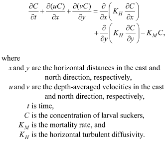
Methods


Larval Datasets


The larval catch data used for this report were collected by three agencies: Oregon State University (OSU), The Nature Conservancy (TNC), and the USGS. Larvae were collected during 4 years between 2006 and 2009 at fixed sites by TNC and OSU and at random sites by TNC. The USGS collected larvae in 2008 and 2009 at fixed and random sites. Twenty‑two fixed sites (fig. 1) were visited multiple times during a season, and were consistent across years, whereas random sites (fig. 2) were visited once and not intentionally repeated within a season. Qualitative differences in the sites visited by the different agencies are apparent. The OSU sites used in this study, with the exception of site W1, were outside of the Delta and close to the shoreline in either Upper Klamath Lake or Agency Lake. The TNC sites were in shallow water (less than 1.0 m deep) either in the Delta or along the levees. The USGS sites were in deeper water than the OSU and TNC sites and consequently farthest from shorelines or levees (primarily within Tulana) and also in Upper Klamath and Agency Lakes across from the levee openings.


Oregon State University data were collected during daylight using a larval trawl (table 1) having a 2.5 m long, 1 mm bar mesh Nitex^® net with a 0.8 × 1.5 m opening mounted on an aluminum frame with runners (LaBolle and others, 1985). The trawl was set 3–12 m offshore in water as much as 1 m deep (range 0.2–1.0 m), allowed to soak for 10 minutes, then pulled to shore with ropes. Sampling from 2006 to 2009 took place the first full week of April through late July, with samples collected at the fixed sites every third week for a total of six sampling surveys. In Upper Klamath Lake, two samples were collected from each of ten fixed sites from 2006 to 2007 (fig. 1). The mouth of the Williamson River changed because of restoration in late 2007. Both the former river mouth site (OSU-W1) and the new river mouth site (OSU-U6) were sampled in 2008 and 2009. In Agency Lake, two samples were collected from each of two fixed sites. Two samples collected at a single site were considered replicates for the purposes of this study. 


The Nature Conservatory data were collected during daylight in pop nets set in water as much as 1 m deep (range 0.1–1.0 m). The nets consisted of two 1 in diameter PVC frames (each approximately 2.56 m²), one weighted with rebar to serve as the lead line and the other wrapped in foam core to act as a float. One-meter wide, fine mesh mosquito netting connected the two frames to form a cube. The nets were open at the bottom and top, allowing them to be set in vegetation. To set the nets, both frames were submerged and secured underwater with two cinderblocks. A long line attached to each cinderblock enabled them to be pulled away from the net without disturbing the sampling area and allowed the foam‑wrapped upper frame to “pop” up, enclosing the section of water. Each net was set for a minimum of 30 minutes prior to sampling to ensure each site had recovered from disturbances resulting from setting the net. Two to four samples were collected at each site, usually within 1 hour of each other. These samples were considered to be replicates for the purposes of this study, although generally one net was set in emergent or submerged vegetation and one was set nearby on substrate with no vegetation, and the depth sometimes varied between the replicate nets.


In 2006 and 2007, pop nets were set in South Marsh and two lakeshore fringe wetlands in Upper Klamath Lake along the Goose Bay shoreline (fig. 2). After restoration in November 2007, the Tulana area of the delta was added to the aforementioned sampling areas for the 2008 sampling period; Goose Bay, after being flooded in October 2008, was added in 2009 (fig. 2). Each sampling area was visited every other week in 2006 and 2008 and weekly in 2007 and 2009. A maximum of eight nets were set at random points within each sampling area each week; however, beginning in 2008 two fixed sites were visited weekly in Tulana and beginning in 2009, two fixed sites were visited weekly in Goose Bay (fig. 1).


The USGS used plankton nets during daylight to collect larvae from the top of the water column. These nets had 0.3 m diameter mouth openings, a 2.5 m long tail, 800 μm mesh Nitex netting, and a removable cod end. A General Oceanics, model 2030R, mechanical flowmeter was mounted in the mouth of each net so that the volume sampled could be calculated. The net was towed parallel to a boat at approximately 1 m/s for 3–5 minutes or until algae began to clog the mesh. After retrieval, all material was meticulously removed from nets and samples were immediately preserved in 70–95 percent ethanol. One, two, or three replicate tows were performed at each site.


The USGS sites consisted of both random and fixed sites. The random sites were selected using a stratified design from deep (greater than 1.5 m) areas in Agency Lake, Tulana, and Upper Klamath Lake, and two shallow (0.5–1.1 m) areas in Tulana (Burdick and Brown, 2010, fig. 2). In 2008, USGS located fixed sites on the lake side of the four breaches that were made in the levees surrounding Tulana (sites 25976, 25977, 25978, and 25979); in open water inside Tulana (site 25980); in about 1 m of water on the east side of Tulana (site 25535); and offshore of the mouth of the Williamson River (site 25981) (fig. 1). In 2009, additional fixed sites were added in the Goose Bay oxbow, nearshore in the western part of Goose Bay, and offshore in the eastern part of Goose Bay (not shown in fig. 1).


Samples collected by each agency were either fixed in 10 percent formalin, and later switched to 50 percent isopropanol for long-term storage, or preserved in 70–95 percent ethanol. Smaller catostomid larvae, less than 14 mm in the OSU catches or less than 15 mm in the USGS and TNC catches, were identified as either Lost River suckers or a grouping of shortnose and Klamath largescale suckers based on pigmentation patterns. Identical protocols were used by all agencies to identify species (Simon and others, unpub. data) and results were cross checked to minimize bias. There is no method for distinguishing between larval shortnose and Klamath largescale suckers. Some suckers had indeterminate patterns and were classified as unidentified suckers. The method of classification of larger catostomid larvae was different at each agency. At TNC, larvae larger than 15 mm were classified as unidentified suckers. At USGS, post-Weberian vertebrae of larvae over 15 mm were counted if they were visible and if the species was in doubt. Those with greater than 44 vertebrae were classified as Lost River suckers, those with less than 44 vertebrae were classified as shortnose/Klamath largescale suckers, and those with 44 vertebrae were classified as unidentified suckers (Markle and others, 2005). At OSU, fish larger than 14 mm were cleared and stained (Potthoff, 1984). Post-Weberian vertebrae were counted on these fish, and species assigned based on post-Weberian vertebral counts as previously indicated. 


Because some samples were fixed in formalin while others were preserved in ethanol, differential larval shrinkage may have introduced some degree of bias in the results. Nominal concentrations were 10 percent formalin and 70–95 percent ethanol, but the inability to make precise mixtures in the field could also contribute to differential shrinkage. Most shrinkage occurs within 1 day and in a study of larval inland silversides, mean shrinkage after 21 days was 3.9–4.1 percent for 80–100 percent ethanol and 2.2–3.2 percent for 5–10 percent formalin (Cunningham and others, 2000). Because the larvae used for otolith ageing followed the methods of Terwilliger and others (2003) and were preserved in ethanol, all measurements include shrinkage from live lengths and age estimates are based on shrinkage of perhaps 4 percent. The 1–2 percent difference in shrinkage between formalin and ethanol is considered trivial for our analyses and no corrections were made. 


Hydrodynamic Model


The UnTRIM hydrodynamic model solves the governing equations for flow and transport on an orthogonal unstructured grid using the efficient and stable algorithms of Casulli and Zanolli (2002). The details of the three-dimensional Upper Klamath Lake model and its calibration and validation for 2005 and 2006 (Wood and others, 2008) are provided elsewhere and not repeated here. A one-layer version of the UnTRIM hydrodynamic model of the lake described in Wood and others (2008) was used in order to speed computation time. The use of a one-layer model removes the effects of water density on the flow, which is not important in the present analysis. In this case, because transport through the Delta is the primary interest, and the flow is expected to be well-described by two dimensions, the benefit of running more simulations in the available time outweighed the loss of accuracy that occurred by using a one-layer model.


The unstructured orthogonal grid used in the UnTRIM model is particularly well-suited to describing the small scale features and complicated boundaries associated with the Williamson River channel and the levees remaining around the channel and the Delta. The elevations within the Delta were obtained from a composite of data interpolated to a grid with 100 ft horizontal spacing (L. Friend, ZCS Engineering, Inc., written commun., 2009). The grid was built from pre‑project survey data, in combination with the engineered design modifications for the project, and then modified with additional surveys to collect data where the design elevations differed from the “as built” elevations. These data were used to generate the bathymetry data in the new Williamson River and Delta parts of the grid, which were then merged into the existing grid for the rest of the lake. Because this study spans the years 2006 through 2009, three versions of the numerical grid were used. A “pre-project” grid was used for 2006 and 2007 simulations. Tulana was flooded in autumn 2007, and therefore a grid that included only that side of the Delta was used for the 2008 simulations. Goose Bay was flooded in autumn 2008, and therefore a grid incorporating both the Tulana and Goose Bay sides of the Delta was used for 2009 simulations (fig. 2). All three grids incorporated the Williamson River channel upstream to the Modoc Point Road bridge (river kilometer 7.4). A Manning formulation was used for the bottom friction in these new areas of the grid. A Manning’s n of 0.026 was used within the channel, to be consistent with a calibrated one-dimensional HEC-RAS model (Graham Matthews and Associates, 2001), and a Manning’s n of 0.05 was used in the Tulana and Goose Bay parts of the Delta, also consistent with Graham Matthews and Associates (2001) and Daraio and others (2004). 


The boundary conditions needed to run the model include wind forcing at the surface and inflows at the Williamson and Wood Rivers, as well as the outflow at the Link River Dam. The wind forcing was obtained from a spatial interpolation of 10-minute data collected at six meteorological sites (fig. 1). Because critical wind data from rafts located on the lake were not always available as early in the spring as required for simulations of larval drift from spawning sites in the Williamson River, some of the wind data from rafts was reconstructed using the artificial neural networks technique described in Buccola and Wood (2010). Missing wind data for May 10–16, 2006, and May 3–9, 2007 were reconstructed using this method. 


The initial lake elevation and the elevations to which model elevations were compared came from three stage gages located around Upper Klamath Lake (fig. 1). Flow information is required at three boundaries: the Williamson River at Modoc Point Road, the Link River at the outlet of Upper Klamath Lake (the Link River Dam), and the Wood River, which empties into Agency Lake. Williamson River and Link River streamflows were obtained from USGS streamflow gaging stations (fig. 1). “Wood River,” as used here, is the sum of inflows at the Wood River channel and two other canal flows, the Fourmile and Sevenmile canals, which are channelized diversions from the Wood River and empty into Agency Lake not far from the Wood River mouth. These flows were not recorded during the time period of this study, except Sevenmile flows in 2006. Flows from all three of these sources were recorded in 2004 and 2005 during May and June (Graham Matthews and Associates, 2009; fig. 1). When the 2004 and 2005 data were combined, the average ratio of those combined flows to the Williamson River flow was approximately 0.6. Therefore, the sum of these flows (Wood River, Fourmile Canal, and Sevenmile Canal) was set to a constant value of 0.6 times the average Williamson River flow for May 15 to June 30 in each year (15.3, 23.0, 10.9, and 28.7 m³/s in 2009, 2008, 2007, and 2006, respectively). The sensitivity of transport through the Delta to the value of the ratio of these flows to the Williamson River flow has been shown to be small (Wood, 2012).


Larval Density Simulations


The hydrodynamic model was used to simulate larval density during the springtime larval drift period of 2006 through 2009. The simulation period was 70 days in each year, starting about 4 days prior to the date when the first significant drift of larvae was observed at the Modoc Point Road bridge. The dates simulated were May 10–July 20, 2006; May 3–July 13, 2007; May 15–July 25, 2008; and May 14–July 24, 2009. 


Williamson River Boundary Condition


Larval-sucker density data collected in the thalweg at the Modoc Point Road (Tyler and others, 2004; Ellsworth and others, 2009) were used to construct the upstream boundary condition for a numerical tracer. Fish captured in the Williamson River drift at the Modoc Point Road were identified as either one of two taxa, Lost River sucker (LRS) or a group of suckers identified as either shortnose or Klamath largescale sucker (SNS/KLS), making it possible to use two tracers to simulate the Lost River and SNS/KLS sucker larvae separately. Fish with indeterminate characteristics were classified as unidentified suckers. The larvae tend to pass the Modoc Point Road bridge in two or more “pulses.” The first pulse is dominated by LRS larvae, and subsequent pulses are dominated by SNS/KLS larvae. Because the larvae are known to drift at night, these drift data were usually collected between about 4–8 hours after sunset, and peaked between about 5–6 hours after sunset. To create a boundary condition, the larval drift data were first multiplied by a factor of 0.39 in order to compensate for higher drift concentrations near the surface and in the thalweg of the river than the average concentration over the cross section, which is the quantity needed for the boundary condition. This value was determined by analyzing cross-sectional larval density data collected at two transects of the Williamson River near Modoc Point Road (Tyler and others, 2004) during the peak nighttime drift hours between 10:00 in the evening and 3:00 in the morning, from May 8 to June 4, 2004 (Ellsworth and others, 2010). The value 0.39 represents a scaling of the cross-sectional area‑weighted average of these larval densities by the larval density measurements taken in the thalweg of the river, where larval sampling occurred in successive years. To provide boundary information each night, gaps that occurred on evenings when crews were not collecting drift data were filled by replicating the data collected during the most recent evening when crews were collecting drift data. Therefore, gaps spanning more than 1 day were filled by repeating the most recent 24-hour drift cycle that was sampled. The resulting concentration data, in units of fish per cubic meter, were applied to water entering the Williamson River boundary in the model grid. Larval drift was collected at intervals ranging from 0.5 to 2 hours; in order to match the 2-minute time step of the model, a measured value was used at every 2-minute time step until a new value was available. At sunrise each day, the boundary condition was set to zero; thus, no larvae were inserted into the model grid between sunrise and sunset. The time series of larval drift and the resulting model boundary condition for 2006–09 are shown in figure 3. 


Larval Transport, Mortality, and Behavior


The model solves the advective-diffusive transport of larval fish using the differential equation:


(1)


A spatially uniform value of 0.1 m²/s for K_H was used in the larval density simulations presented in this report, corresponding to velocity and length scales of turbulence of 0.1 cm/s and 100 m, respectively.


According to Houde and Zastrow (1993), the mean mortality rate for the larval stage of marine fish is K_M = 0.24, resulting in a loss of 21.3 percent of the population each day. For freshwater fish larvae, the rate is somewhat lower, at 14.8 percent each day, presumably because most of the species studied hatch from large eggs (Ware, 1975; Houde and Zastrow, 1993). A crude approximation of larval stage mortality rate K_M also can be derived from growth rates (K_G), using K_M = 1.217* K_G – 0.0131 (Houde and Bartsch, 2009). Using the larval age and length data set from Markle and others (2009), the approximations are strongly size dependent, as expected (Houde and Bartsch, 2009). First-order estimates for sucker larvae by Markle and others (2009) were 8.2 percent each day for SNS/KLS suckers (K_M = -0.0857 d^-1) and 2.6 percent each day for Lost River suckers (K_M = -0.0262 d^-1). Given the variability in these mortality estimates, the size-dependent function of mortality, and the focus of this study on young larvae entering the lake, a somewhat higher K_M of 0.1 d^-1, corresponding to a loss of just over 10 percent of the population each day, was used. 


The larval drift data collected in the Williamson River show that drift occurs at night, and that the larvae drop out of the flow, presumably holding position either near the bottom of the channel or at the sides of the channel during the day (Cooperman and Markle, 2003; Ellsworth and others, 2009). This behavior was incorporated into the larval density simulations as follows: At sunrise on each day, the larvae in each polygon of the Williamson River channel part of the numerical grid were removed. At sunset on each day, the same number of larvae that were removed from each Williamson River polygon on the previous sunrise was added back to that polygon. Any larvae that moved into the Williamson River polygons from the surrounding areas after sunrise were not stored and were transported normally throughout the day. The behavior was the same for both species.


The persistence (downstream distance or length of time) of this behavior—moving vertically or horizontally within the channel to escape the current during the day—is uncertain, and likely is age and (or) habitat dependent (Leis 2007; Gerlach and others, 2007; Wright and others, 2011). Three possible cases were considered: (1) The nighttime-only drift behavior was simulated through the entire Williamson River channel between the upstream boundary at Modoc Point Road and the mouth at Upper Klamath Lake, (2) The nighttime-only drift behavior was simulated in the Williamson River channel only upstream of the point where the channel enters the flooded land of the Delta (fig. 2), and (3) The nighttime-only drift behavior was assumed to occur only upstream of the Modoc Point Road boundary, and was not simulated in the channel within the domain of the numerical model.


Comparison to Larval Catch Data


Simulated larval densities were compared directly to larval catch data. Data from both randomly selected and fixed sites were included in this analysis. At each geographic location and time that a net measurement was made, the simulated density of larvae in the grid polygon associated with the site location (fig. 2), and at the time corresponding to the net catch, was paired with values of observed larval density in the net. For this purpose, replicate net measurements were averaged. Fish densities were not normally distributed, and a rank order correlation coefficient (Spearman ρ) was calculated for the paired data. Ties in the ranked data were assigned the same averaged rank.


Correlations were calculated for the simulation period in each year by combining data collected in all gear types and by separating data collected in pop nets, larval trawls, and plankton nets. Additionally, the larval catches from each gear type were separated into small (10 to 13 mm), mid (greater than 13 to16 mm), and large (greater than 16 to19 mm) sized fish, and the correlations were calculated for each size class. Using 2009 data only, the plankton net and larval trawl data were separated by species into LRS and SNS/KLS, and the correlations were calculated for each species. Finally, using 2009 data only, the correlations were calculated for each size class, with simulated data based on three assumptions regarding the spatial extent of Williamson River drift: throughout the channel from Modoc Point Road to the mouth, upstream of the Williamson River Delta only, and upstream of Modoc Point Road only.


First posted April 2, 2012