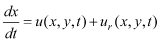
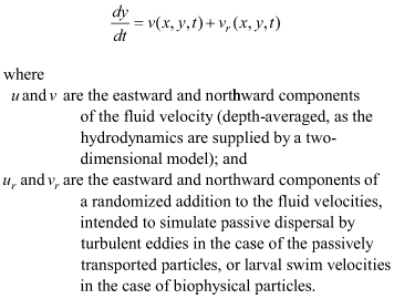
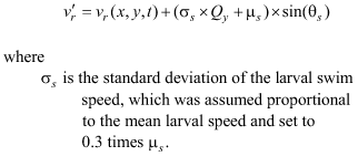
Methods


Larval Datasets


Oregon State University (OSU), The Nature Conservancy (TNC), and the U.S. Geological Survey (USGS) collected larval catch data in 2009 at both “fixed” sites and “random” sites. Multiple visits to 22 fixed sites (11 OSU sites, 4 TNC sites, and 7 USGS sites; fig. 1) were selected for comparison of simulated results to larval catches, and to describe the spatial pattern of the distribution of simulated particle ages and lengths. Random sites were visited only once per season. Data from fixed (fig. 1) and random sites were combined (fig. 2) for correlating simulated results with larval catches. Most of the OSU sites were located outside the delta and close to lake shorelines. The TNC sites were located in shallow water (less than 1.0 m deep) in the delta and along the levees. The USGS sites were located in deeper water than the OSU and TNC sites and, therefore, were farthest from shorelines or levees.


Larval data collection and preservation methods are described in detail in Wood and others (2012), and are only briefly described here. Data were collected by OSU during daylight hours with a larval trawl (LaBolle and others, 1985) set close to shore in water up to 1 m deep. Samples were collected from early April through late July every third week for a total of six sampling surveys. Two replicate samples were collected from each of the 11 OSU fixed sites used in this work (fig. 1). 


Data were collected by TNC during daylight hours, with 2.56-m² pop nets set in water as much as 1 m deep. Two to four “replicate” samples were collected at each site, usually within an hour of each other. The samples were considered replicates for this study even though one net might have been set in emergent or submerged vegetation while another net nearby might have been set on substrate with no vegetation, and the depth also sometimes varied between the replicate nets. Four fixed sites were visited weekly, two in the northern delta and two in the southern delta (fig. 1) along with the random sites (fig. 2).


USGS used diurnal plankton net tows to collect larvae from the top of the water column by towing the net parallel to a boat at approximately 1 m/s for 3–5 min or until algae began to clog the mesh. One, two, or three replicate tows were done at each site. Plankton net samples used in this study were collected at random sites (fig. 2) and at seven fixed sites (fig. 1).


USGS also collected samples at the upstream bounary site of the model (fig. 2), which is at Modoc Point Road Bridge, 7.4 river kilometers upstream of the historical mouth of the Williamson River. Samples were collected from the thalweg by deploying a weighted plankton net equipped with a flow meter from the bridge for 10-min sets. Samples were collected from March 23 to July 17, three times each week, between sunset and 5–8.25 hours after sunset. Additional sampling details are in Ellsworth and others (2009).


Samples were either fixed in 10-percent formalin and later transferred to 50-percent isopropanol or preserved directly in 70–95-percent ethanol. Because some samples were initially fixed in formalin and others were placed directly into ethanol, differential larval shrinkage may have introduced some bias in the results. However, the 1–2 percent difference in shrinkage between formalin and ethanol was considered trivial for our analyses and no corrections were made. Larval species were identified according to methods described in Wood and others (2012).


Larval Age Data and Application to Simulations


Sampling methods targeted larvae-sized fishes, so to reduce problems with reduced gear efficiencies for larger larvae, all analyses were restricted to larvae with a standard length (total length minus tail length) of 10–19 mm. All references to fish lengths used in this study refer to standard lengths. We aged 112 sucker larvae with lengths between 11.5 and 19.0 mm from the 2009 TNC samples (Erdman and Hendrixson, 2010), following the methods of Terwilliger and others (2003). The age estimate (in days) of each larva was based on median lapillus otolith ring counts from three blind reads by the same reader of each otolith. The resulting relation between length and age was age = 4.55 × length – 44.86 (coefficient of determination [R²] = 77.1 percent) where length is the standard length of the fish in millimeters, and age is the estimated age of the fish in days. The intercept is near or within the range of hatch sizes reported for Lost River suckers (9.6–10. 4 mm) and shortnose suckers (7.0–9.6 mm) (Hoff and others, 1997). The equation for age as a function of length was converted to a length-at-age relation (length = 9.87 + 0.22 × age; fig. 3) in order to determine the swim speed associated with individual particles within the model and to convert particle ages to lengths for comparison to field data.


The age of all particles was assumed the same at the time of insertion into the model grid, and was determined as the sum of the age at the Modoc Point Road Bridge and the travel time between the bridge and the location where particles were inserted into the grid (fig. 2). The estimated age (8.3 d) at the Modoc Point Road Bridge was calculated from the median standard length (11.7 mm; Ellsworth and Martin [2012]) of 8,695 sucker larvae caught there, using the regression equation for age as a function of length, age = 4.55 × length – 44.86. Travel time between the Modoc Point Road Bridge and the domain boundary was determined with numerical travel time experiments in which a tracer, simulating nighttime larval sucker behavior, was initialized at the Modoc Point Bridge and allowed to travel down the Williamson River channel. The travel time experiments used the range of streamflows measured between May 18 and June 7, 2009, the span of time during which most of the particles were inserted. Travel time was 1.0 d, resulting in an initial age of 9.3 d for each particle inserted into the simulation.


The span of inference for the model was limited to fish aged less than 46 d (20 mm standard length, based on the length-at-age relation). The 20-mm standard length and 46-d limit correspond to an age when most individuals would be approaching the juvenile stage. Given these considerations, particles were tracked individually from 9.3 d of age until they either left the domain through the outflow boundary at the Link River (fig. 1) or reached 46 d of age. Therefore, the maximum time that a particle was tracked in the model domain was 36.7 d. Retention of particles in the lake was measured by calculating the ratio of the number of particles that had left the domain at the Link River at the end of the simulation to the number that had reached the 46-d age limit (R_E/A).


Swim speed is a function of fish length, and several relations were used to determine model inputs. The maximum burst speed for razorback sucker larvae with a standard length of 19 mm has been determined to be 464 mm/s or 24 body lengths (BL) per second (BL/s) (Wesp and Gibb, 2003). Prolonged swim speeds (50 percent of fish held this speed for 1 hr) were determined to average 5.8 BL/s (range of 5.3 to 6.5 BL/s) for robust redhorse sucker larvae with a standard length of 13.1–20.4 mm (Ruetz and Jennings, 2000). No historical observations on sustained cruising speeds (speeds that can be maintained indefinitely) were found for larval suckers. However, herring and anchovy larvae are similarly elongate, and their sustained speeds are well documented and potentially comparable to sucker larvae. Using the regression in Blaxter and Hunter (1982), larvae with a standard length of 10–19 mm would have sustained cruising speeds of 1.2 BL/s. Therefore, an intermediate speed of 3.5 BL/s was chosen for most simulations and sensitivity to swim speed was investigated using sustained (1.2 BL/s) and prolonged swim speeds (5.8 BL/s). Swim speeds were applied by converting particle ages to body length using the length-at-age regression and calculating swim speed from body length.


Mortality is strongly size-dependent and difficult to measure in larval fishes (Houde and Bartsch, 2009). According to Houde and Zastrow (1993), the mean mortality rate (K_M) for freshwater fish larvae is 14.8 percent per day. First‑order estimates for sucker larvae from the Upper Klamath Lake, which are longer than many freshwater fish larvae at hatch, ranged from 8.2 to 2.6 percent per day (Markle and others, 2009). Because of the variability in these estimates, an intermediate K_M was used that corresponded to a loss of 5 percent of the population each day (K_M=0.051/d).


Hydrodynamic Model


The UnTRIM hydrodynamic model solves the governing equations for flow and transport on an orthogonal unstructured grid using the efficient and stable algorithms of Casulli and Zanolli (2002). The details of the three-dimensional Upper Klamath Lake model and its calibration and validation are provided for 2005 and 2006 in Wood and others (2008). The one-layer version of the hydrodynamic model that was used in this study, including determination of the flow boundary conditions at the tributaries and the lake outlet, and initialization of the lake elevation, is described in Wood and others (2012). The wind forcing at the surface of the lake was obtained from a spatial interpolation of 10-min data collected at six meteorological sites, and the elevation of the lake was determined as a weighted average of three stage gages on the shoreline (fig. 1). Three versions of the numerical grid were used in this study to investigate the sensitivity of travel times to the shoreline configuration: (1) prior to the start of restoration, (2) after the first phase was completed (reconnection to the lake of the northern part of the delta only), and (3) after restoration was complete (reconnection of both the northern and southern parts of the delta).


Simulated Larval Behavior


To simulate sucker larvae, numerical particles were inserted into the model domain and tracked individually from the time they were inserted until they either left the domain through the outflow boundary at the Link River (fig. 1) or reached 46 d of age, the span of inference for our model. Simulations spanned the period May 14–July 24, 2009. Dispersal of particles was simulated assuming passive dispersal and three types of active dispersal with swimming behavior.


Boundary conditions for a numerical tracer entering the delta were based on larval sucker-density data collected in the thalweg at the Modoc Point Road Bridge using the method described in Wood and others (2012). Particles representing individual larvae were inserted along a transect across the river channel, about 175 m upstream of the point where the channel enters the delta (fig. 2). At each model time step, the concentration of the tracer representing larval density was determined at the center of this transect, and the number of particles inserted into the model domain at that time step was in constant proportion to the tracer concentration. Using this method, 3,748 particles were inserted during the 70-d simulation in 2009, with a temporal pattern that mimicked the temporal pattern of the total density of sucker larvae in the drift at Modoc Point Road (Ellsworth and Martin, 2012). (“Drift” refers to the organisms suspended in the current of a stream.) Each dispersal scenario was simulated four times, and the particles were combined, so that nearly 15,000 particles were used to calculate travel times and to compare with field data for each scenario.


The application of fish behavior to larval fish dispersal models is complex (Leis, 2007), and, without specific information on swimming orientation and sensory abilities, we used a simplified approach that was designed to explore how different types of swimming behavior would be manifested in the larval dispersal patterns. Nighttime drift behavior was applied only to particles in the channel of the Williamson River. Lacking specific knowledge of environmental stimuli that trigger nighttime drift, particles in the channel were held in place from sunrise to sunset and tracking was resumed at sunset.


Horizontal swimming was incorporated as both non‑oriented (randomized) and oriented swimming. Advective transport was determined by the sum of the depth-averaged velocity provided by the model simulation and a random component intended to mimic swimming behavior. Simulation of swimming required swim speed, µ_s, the length of time during which the speed was maintained before a change in direction occurred, τ_s, and the angle of the swim vector, θ_s. Swim speed was a function of length, which was determined from the length-at-age regression.


Oriented swimming in fish larvae can be complex, often highly directional, and may or may not be influenced by cues such as light, currents, or shorelines (Trnski, 2002; Leis and Carson-Ewart, 2003). In this study currents simulated by the hydrodynamic model were used as cues. The swimming direction in some fish larvae is not influenced by current direction (Leis and Carson-Ewart, 2003), but it can be in some species and life stages (Champalbert and Marchand, 1994). Because there is evidence that larval retention in the lake, and presumably in the delta, is an important predictor of juvenile recruitment success (Markle and others, 2009), the effect of rheotaxis on biophysical retention was investigated. Oriented swimming was simulated as a tendency by the fish to swim at an angle approximately aligned with the current and directed downstream with the current. Oriented swimming was simulated to occur only at night (between sunset and sunrise). Lacking information on larval fish, oriented swimming was defined to occur at current speeds greater than or equal to 5 cm/s, which was the threshold determined for rheotaxic behavior in juvenile sole with a standard length of 9–14 mm (Champalbert and Marchand, 1994). The angle of swimming θ_s changed on a time step equal to the time step of the hydrodynamic model, such that τ_s was equal to 2 min.


Particle Tracking


The particle-tracking algorithm that was used to track both passive and biophysical particles has the general form:


       (1)


and


(2)


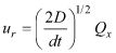
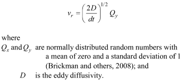
The particle tracking equations were solved using the same time step that was used in the hydrodynamic model to update the advective velocities (2 min). 


For passive dispersal, which is designated scenario A, the randomized components are based on a two-dimensional random displacement model in which the eddy diffusivity is constant:


       (3)


(4)


In practice, the random numbers are calculated from two other random numbers uniformly distributed from 0 to 1 using the Box-Muller transformation (Box and Muller, 1958). When particle tracking carried a particle across a solid boundary, a new pair of random numbers Q_x and Q_y were chosen and a new set of the components u_r and v_r were calculated, until the particle tracking did not result in the particle being carried across a solid boundary. This was attempted up to 100 times, at which point the particle was considered “lost” and was no longer tracked, but very few particles were lost in this way. Eddy diffusivity, D, was set to a value of 0.1 m²/s, consistent with the value used in the advection-diffusion approach of Wood and others (2012).


Active dispersal was simulated in scenarios B, C, and D. In these scenarios, swimming behavior was simulated by replacing the randomized components of velocity for passive particles with components in the form:


       (5)


and


       (6)


In simulations of dispersal that included nighttime-only drift behavior, if the particle was in the Williamson River channel between sunrise and sunset, the particle was not allowed to move, in order to simulate nighttime-only drift. Two types of swimming behavior were simulated by the choice of θ_s. 


For scenarios B and C, which assumed random swimming, the direction of swimming θ_s was randomly chosen from a uniform distribution between – π and π. In the oriented swimming scenario D, the angle of the water current θ_c at the starting position of the particle was determined at the beginning of each tracking step. Oriented swimming occurred only between sunset and sunrise and only when the current speed was greater than 5 cm/s. During the day and anywhere that the current speed was less than 5 cm/s, swimming was non-oriented. When swimming was oriented, swim direction was sampled from a von Mises distribution (Best and Fisher, 1979) centered on θ_c that provided a moderate preference for alignment with the current (approximately 75 percent of the distribution was within ±30° of θ_c –π and 97 percent of the distribution was within ±60° of θ_c –π). If particle tracking carried a particle across a solid boundary, it was retained at the shoreline for that time step, and not moved. At the next time step, tracking of all particles, including those retained at the shoreline, resumed as usual. Therefore, when swimming behavior was simulated, particles were never “lost” from the simulation. 


Movement in the Williamson River channel was assumed to occur throughout the day in scenario B, but was assumed to occur only at night in scenarios C and D. Nighttime-only drift was simulated in scenarios C and D by storing the location of any particles in the Williamson River channel at sunrise. Tracking of those particles stopped at sunrise and resumed at sunset.


Sensitivity of Travel Times to Lake Elevation and Shoreline Configuration


Dispersal scenario C was used to investigate the effect of lake elevation on particle dispersal through the delta and travel times by simulating two additional initial lake elevations. The first additional initial elevation was 0.19 m higher than the recorded initial elevation, which meant that the lake was at full pool at the maximum elevation achieved during the simulation (scenario C+). The second additional initial elevation was a similar distance (0.25 m) lower (scenario C-) than the recorded starting lake elevation, which was 1,262.7 m above the Upper Klamath Lake Vertical Datum. Subsequent changes in lake elevation relative to the starting elevation were identical for scenarios C, C+, and C-. Scenarios C+ and C- each were simulated once, so 3,748 particles were used to calculate travel times for each of these scenarios.


Dispersal scenario C also was used to better understand the changes in particle dispersal attributable to changes in the shoreline that occurred as restoration proceeded between 2007 and 2009. To do this, all boundary and forcing conditions remained as observed in 2009, but simulations of particle tracking were completed for the shoreline configuration as it existed in 2007 (before restoration, scenario C-2007) and 2008 (northern delta only flooded, scenario C-2008). The results of C-2007 and C-2008 were compared to the simulation completed for the shoreline configuration as it existed starting in 2009 (northern and southern parts of the delta flooded, scenario C). Scenarios C-2007 and C-2008 each were simulated once, so 3,748 particles were used to calculate travel times for each of these scenarios.


Travel Times, Conversion to Length, and Comparison to Larval Catch Data


The median travel times to the fixed larval catch sites (fig. 1) were determined by sampling the particles in the simulation every 6 hr. All particles located within a circle of radius 75 m centered on each fixed site were identified, and the ages of those particles were compiled. All particle ages compiled at each site were combined to create a travel-time distribution at that site, and the median value was determined.


To compare model simulations to field data, particle ages were first converted to fish standard lengths using the length-at-age relation. All references to simulated lengths used in this study refer to standard lengths. Then, mortality was applied to the particles as a post-processing step, at a rate of 0.051/d. To simulate mortality at this rate, 5 percent of the particles in the domain at midnight on each simulation day were randomly chosen and deleted from that time forward. The process was repeated for each simulation day. The median lengths at the fixed larval catch sites (fig. 1) were determined by sampling the particles remaining in the simulation after mortality was applied and combining all particle lengths collected at each site to create a length distribution at that site. Simulated length distributions were compared graphically to the larval catch length distributions (all sample dates combined) at the fixed sites where at least 10 suckers were captured during the season. 


Simulated particle lengths were compared to the lengths of fish captured in individual nets at random and fixed field sites by pairing field and simulation data, and calculating a linear correlation coefficient. All particles located within a 150 m radius of a field site, up to 1 hour before and after net sampling, were identified and their median age was calculated. The set of paired values of particle and larval median lengths were compared using a Pearson R correlation coefficient for each swimming scenario. This analysis was done with larval catches from all gear types combined and with larval catches from each of the three gear types separated. This analysis also was done by separating larval catches (all gear types combined) into small (fish length <13 mm), medium (fish length ≥13 mm and <16 mm), and large (fish length ≥16 mm and ≤19 mm) fish. The correlation analysis also was done separately for particles inserted into the domain prior to and after June 2 in order to analyze separately particles representing (predominantly) Lost River sucker larvae prior to June 2 and (predominantly) shortnose sucker larvae after June 2.


First posted January 31, 2014