Scientific Investigations Report 2017-5118
By David B. Smith, Federico Solano, Laurel G. Woodruff, William F. Cannon, and Karl. J. Ellefsen
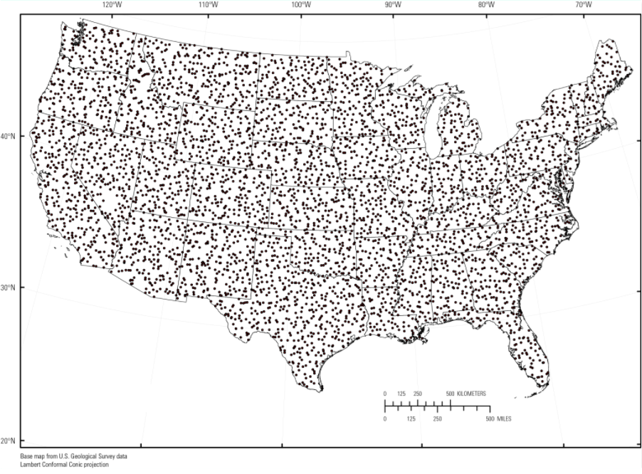
Figure 1. Location of sample sites.
Between 2007 and 2013, the U.S. Geological Survey conducted a low-density (1 site per 1,600 square kilometers, 4,857 sites) geochemical and mineralogical survey of soils in the conterminous United States. The sampling protocol for the national-scale survey included, at each site, a sample from a depth of 0 to 5 centimeters, a composite of the soil A horizon, and a deeper sample from the soil C horizon or, if the top of the C horizon was at a depth greater than 1 meter, a sample from a depth of approximately 80–100 centimeters. The <2-millimeter fraction of each sample was analyzed for a suite of 45 major and trace elements by methods that yield the total or near-total elemental concentration. The major mineralogical components in the samples from the soil A and C horizons were determined by a quantitative X-ray diffraction method using Rietveld refinement. This report presents all the maps and statistical information for each determined element and mineral along with an interpretive section discussing the possible processes that caused the observed national-scale geochemical and mineralogical patterns. Most often, the geochemical and mineralogical patterns reflect the composition of the underlying soil parent material with some modifications caused by leaching of the more mobile elements (for example, calcium and sodium) in the humid areas of the country.
Between 2007 and 2013, the U.S. Geological Survey (USGS) conducted a low-density (1 site per 1,600 square kilometers (km2), 4,857 sites; see fig. 1) geochemical and mineralogical survey of soils in the conterminous United States. The sampling protocol for the national-scale survey included, at each site, a sample from a depth of 0 to 5 centimeters (cm, termed the top 0- to 5-cm layer throughout the website), a composite of the soil A horizon, and a deeper sample from the soil C horizon or, if the top of the C horizon was at a depth greater than 1 meter (m), a sample from a depth of approximately 80–100 cm (fig. 2). The <2-millimeter (mm) fraction of each sample was analyzed for a suite of 45 major and trace elements by methods that yield the total or near-total elemental concentration. All samples from the soil A and C horizons were analyzed by X-ray diffraction (XRD) and the percentages of major mineral phases were calculated by a Rietveld refinement method. Complete geochemical and mineralogical data along with details on the sampling methods, analytical techniques, and quality control protocols are available in USGS Data Series 801 (Smith and others, 2013, available at https://pubs.usgs.gov/ds/801/.
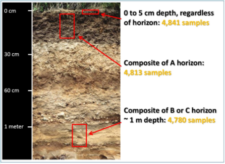
Figure 2. Soil profile showing sampling depths.
USGS Open-File Report 2014-1082 (Smith and others, 2014, available at https://pubs.usgs.gov/of/2014/1082/, accessed August 8, 2017) contains geochemical and mineralogical maps along with a histogram, boxplot, and empirical distribution function plot for each element or mineral. In the maps, the spatial distribution of each element or mineral is shown either by an interpolated and smoothed average color surface map or a proportional symbol map. Color classes were chosen by the authors using percentiles of the analytically determined values for each element and mineral. The interpolated grid cell values are thus portioned into 10 classes as follows: 0–10th percentile, 10th–20th percentile, 20th–30th percentile, 30th–40th percentile, 40th–50th percentile, 50th–60th percentile, 60th–70th percentile, 70th–80th percentile, 80th–90th percentile, and 90th–100th percentile. Each class is represented by a unique color, ranging from blues (lowest concentrations) to reds (highest concentrations). Thus, each class and color represents approximately 10 percent of the data. Elements and minerals that were detected in fewer than 30 percent of the samples are shown on the maps as proportional symbols rather than an interpolated surface. For approximately half of the geochemical maps, a small number of selected high concentrations (one to six) were removed prior to the inverse distance weighting (IDW) interpolation. Those high concentrations likely represent a point source of either natural or anthropogenic origin and are not representative of a larger region. If included in the interpolation, they produce an unrealistically large area of predicted high concentrations and unduly affect the classification of values used in the display. All the removed samples are shown as points (diamond symbols) on the interpolated maps along with their element concentrations. A more detailed explanation of the generation of the maps and statistics is given in Smith and others (2014).
The purpose of this online report is to present all the maps and statistical information given in Smith and others (2014) along with an interpretive section for each element and mineral discussing the possible processes that caused the observed national-scale geochemical and mineralogical patterns.
The Top Menu has four permanent options:
Clicking on any mineral or element from the Mineralogy or Geochemistry links takes the user to a map visualization for that mineral or element. On each map page, to the right of the map are three rhomboids representing the three sample types collected in this study—top 0- to 5-cm layer, soil A horizon, and soil C horizon. For the mineralogical maps, the rhomboid representing the top 0- to 5-cm layer is not active because mineralogy was not determined for this sample type. This is also true for forms of carbon (C); although the rhomboid for the top 0- to 5-cm layer seems active, no map is actually shown as carbon was not analyzed for this sample type. Clicking any of the rhomboids opens the maps for that sample type. Additional options are presented through buttons placed below the sample type rhomboids shown. These options include:
Clicking this button displays a brief interpretive discussion of the mineralogical or geochemical patterns observed for the selected mineral or element.
The interpretive discussions provide a perspective on the observed regional- and national-scale variations in element and mineral distributions in soils and their likely causes. The significant spatial variations shown by most elements can commonly be attributed to geologic sources in underlying soil parent materials, but other spatial variations seem clearly related to additional factors such as climate, the age of soils, transported source material, and anthropogenic influences. This report distinguishes, as much as feasible, the influence of these various factors on a regional and national scale. Many local-scale features might similarly be related to these same factors, but these features also have some probability of being an artefact of a random sampling of soils of variable compositions. There is, therefore, some probability of samples with similar compositions occurring in clusters of two or more adjacent sites by chance. Distinguishing such random occurrences from variability related to soil-forming processes is beyond the utility of the data from which these maps are constructed. Some caution, therefore, is advisable in interpreting the significance of these more local features unless some unique sources or processes can clearly be related to them.
Within each discussion are a number of features to make the interpretation more interactive and explanatory. For example, hovering the mouse over any colored text will trigger the following types of information:
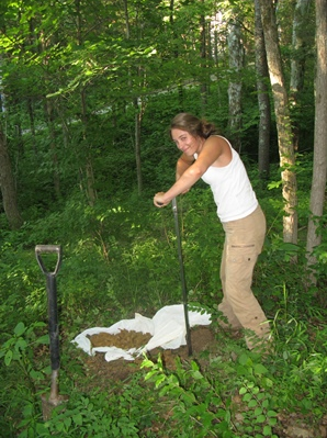
Photograph by Helen Whitney, USGS.
When the user clicks on the STATISTICS button, a table and three graphics (histogram, boxplot, and empirical cumulative distribution function) are displayed for the corresponding sample type. In the table, the median absolute deviation (MAD) and the robust coefficient of variation (robust CV) were calculated for all elements except those where more than 5 percent of the analyzed samples had concentrations below the lower limit of determination (LLD). (Throughout this report, LLD represents lower limit of determination or lower limit of detection, as applicable.) The MAD was scaled by 1.4826 for asymptotically normal consistency (Reimann and others, 2008). The plots were generated with the R statistical computing environment (R Core Team, 2013). Each of these graphics, in its own way, allows the determination of whether the data distribution is symmetric or skewed, unimodal or multimodal, and whether data outliers are present at either extreme of the distribution. The horizontal axis (concentration) is arithmetic except for some elements or minerals where the distribution is highly right-skewed. In those cases, a logarithmic scale is used. For the histograms, the bin widths are determined by the Sturges formula (Sturges, 1926) when the horizontal axis is arithmetic and by the range of the log-transformed data when the horizontal axis is logarithmic. Each graph shows the LLD as a red vertical dashed line. Concentrations that are less than the LLD have been set to a value of one-half the LLD for the graphics. For some elements or minerals (for example, silver, Ag), a large percentage of the data is below the LLD; this results in highly distorted plots. The table and boxplot are also included as an overlay activated in the interpretation texts (look for the words 'summary statistics,’ and hover the mouse to display them).
Three download buttons related to the mineral or element displayed on the map are available for increased functionality:
In preparing the interpretive text for each element and mineral, we cite uses of that element or mineral and typical concentrations of each element in different rock types to illustrate the range of concentrations that can be found in soil parent material. We also cite the chemical formulas for several minerals. Many information sources were used. Rather than interrupt the text with so many citations, we have chosen to list the various sources here:
The pictures that accompany interpretive texts of minerals are used with permission from two sources: the Smithsonian Institution (click here to access the Smithsonian Institution National Museum of Natural History GeoGallery website, and download images of rocks, minerals, gems, and meteorites) and from the collection of images by Roger N. Weller, maintained at the Cochise College Virtual Geology Museum (click here to visit that site and access more images of minerals, rocks, and fossils).
Thanks to Juan Pablo Solano, WonderCraft, who was instrumental in developing the design concept for this website. Steve Smith and Helen Whitney (USGS) provided thoughtful and thorough reviews that greatly improved the manuscript.
Many people contributed to the success of this project. Obviously, the collection of samples from 4,857 sites across the conterminous United States was a difficult undertaking that would not have been possible without the hard work of many people. U.S. Geological Survey personnel who assisted with sampling included Jim Kilburn, Damon Bickerstaff, Helen Whitney, Harley King, John Horton, Suzanne Nicholson, and Klaus Schulz. From 2008 to 2010, the project employed students from universities throughout the United States to collect samples. The project could not have been completed without the outstanding contributions of the following: Kevin Bamber (University of Missouri), Samantha Bray (University of Nebraska), Joseph Daniel (North Carolina State University), Travis Drier (University of Wisconsin, Platteville), David Eaton (Utah State University), Josh Edgell (North Carolina State University), Stephanie Fish (University of Minnesota), Daniel Johnson (Virginia Polytechnic Institute and State University, popularly known as Virginia Tech), Shawn Koltes (North Dakota State University), Michael Marsicano (Delaware Valley College), Robert Matthews (University of Missouri), Jazelle Mondeau (University of Arizona), Robert Moore (North Carolina State University), Laura Murphy (University of Wisconsin, River Falls), Nina O'Malley (Virginia Tech), Jonathan Parr (University of Arizona), Lindsay Shirk (Delaware Valley College), Adam Stevens (University of Southern Maine), and Daniel Vogelsang (University of Missouri).
U.S. Department of Agriculture (USDA) Natural Resources Conservation Service (NRCS) personnel in North Dakota and South Dakota collected all the samples in those states. The Minnesota Geological Survey, the Pennsylvania Geological Survey, and the University of Nebraska's Conservation and Survey Division collected samples in their respective states. We thank the individuals who coordinated the work (Harvey Thorleifson, Minnesota; Steve Shank, Pennsylvania; and Mark Kuzila, Nebraska) and all those who participated in sampling in these three states.
Jaime Azain and David Detra (USGS) oversaw the huge task of disaggregating, grinding, and splitting the samples; shipping the samples to the laboratory; and archiving the samples. Their capable staff included Murray Beasley and David Walters (USGS), Devon McGillivary (Pathways Program intern), and Rene Krine (contractor). Tiffani Schell (USGS) was responsible for sample preparation for XRD analyses and for the instrumental measurement of diffractograms. Helen Whitney and John Jackson (USGS) assisted in X-ray analyses through advice on techniques and interpretations, quality control procedures, and identification of clay phases.
We would like to especially acknowledge Jim Kilburn (USGS) for his tireless efforts on this project. Jim not only collected samples in various States, he also (1) trained most of the students in the USGS sampling protocols; (2) received and catalogued the more than 14,000 samples as they arrived from the field; (3) oversaw the drying of the samples; and (4) prepared all the paperwork for submitting the samples to the laboratory for chemical analysis.
We are also grateful for the support of the Directors and Acting Directors of the USGS as well as the Mineral Resources Program Coordinators who served during the project's lifetime. Lastly, we would like to say thank you to all the landowners who generously gave us permission to take soil samples from their property. The project could not have been completed without their cooperation.
U.S. Department of the Interior
DAVID BERNHARDT, Secretary
U.S. Geological Survey
James F. Reilly II, Director
U.S. Geological Survey, Reston, Virginia: 2019
For more information on the USGS—the Federal source for science about the Earth, its natural and living resources, natural hazards, and the environment—visit https://www.usgs.gov/ or call 1–888–ASK–USGS (1–888–275–8747).
For an overview of USGS information products, including maps, imagery, and publications, visit https://store.usgs.gov/.
Any use of trade, firm, or product names is for descriptive purposes only and does not imply endorsement by the U.S. Government.
Although this information product, for the most part, is in the public domain, it also may contain copyrighted materials as noted in the text. Permission to reproduce copyrighted items must be secured from the copyright owner.
Suggested citation:
Smith, D.B., Solano, Federico, Woodruff, L.G., Cannon, W.F., and Ellefsen, K.J., 2019, Geochemical and mineralogical maps, with interpretation, for soils of the conterminous United States: U.S. Geological Survey Scientific Investigations Report 2017-5118, https://doi.org/10.3133/sir20175118. [Available as HTML.]
ISSN 2328-0328 (online)
Publishing support provided by the Science Publishing Network,
Denver Publishing Service Center. Report website development, coding, and 508 compliance was provided by Bobbie Jo Hanks, USGS.
For more information concerning the research in this report, contact the
Center Director, USGS Geology, Geophysics, and Geochemistry Science Center
Box 25046, Mail Stop 973
Denver, CO 80225
(303) 236-1800

![]() U.S. Department of the Interior |
U.S. Geological Survey
U.S. Department of the Interior |
U.S. Geological Survey
URL: http://pubsdata.usgs.gov/pubs/sir/2017/5118/index.html
Page Contact Information: GS Pubs Web Contact
Page Last Modified: Wednesday, 24-Apr-2019 13:10:48 EDT
