During the course of this study (1986-1995), 25 debris flows occurred in Grand Canyon (Melis and Webb, 1993; Melis and others, 1994; Webb and Melis, 1995; Webb and others, unpublished data). For as many of these events as feasible, we traced the debris flow to its initiation point to evaluate the failure mechanism and source material. Using other reports (for example, Cooley and others, 1977), we augmented our data with data on other notable, historic debris flows.
We obtained climatic data from the National Climatic Data Center in Asheville, North Carolina, and from their reports (for example, NOAA, 1996). We used daily rainfall data, and we calculated storm precipitation by summing over consecutive days with rainfall preceding historical debris flows. We estimated the probability of daily and storm precipitation using the modified Gringorten plotting position (U.S. Water Resources Council, 1981),
| p = ((m - 0.44)/(n + 0.12)) • d, | (1) |
where p = probability of the event, m = the ranking of the event, n = the number of days in the record, and d = the number of days in the season per year. The recurrence interval, R (yrs), is
| R = 1/p. (2) | (2) |
Melis and others (1994) identified 529 geomorphically significant tributaries to the Colorado River in Grand Canyon from Lees Ferry to Diamond Creek, excluding the four largest tributaries (the Paria and Little Colorado Rivers, and Kanab and Havasu Creeks). They selected tributaries that have the potential to produce debris flows that affect the geomorphology of the river channel. Their criteria include: 1) drainage areas larger than 0.01 km2; 2) mapped perennial or ephemeral streams; 3) previously designated official name; 4) clear termination at the Colorado River in a single channel; 5) formation of obvious debris fans and (or) rapids. We extend these definitions to 71 additional tributaries between Diamond Creek and Surprise Canyon in western Grand Canyon (river miles 225 to 248).
Although there are a variety of possible methods for dating recent debris flows, including the 3He, 14C, and 137Cs techniques (Hereford and others, 1996; Melis and Webb, 1993; Melis and others, 1994; Webb and others, 1996), the most useful method in Grand Canyon is repeat photography for historic events (Webb, 1996). Repeat photography has been used to identify changes in plant distributions, effects of operations of Glen Canyon Dam on sand bars, and the appearance of debris-flow and flood deposits in previous studies in Grand Canyon (Turner and Karpiscak, 1980; Stephens and Shoemaker, 1987; Webb and others, 1988, 1989; Melis and others, 1994; Schmidt and others, 1996; Webb, 1996). This success is in large part due to the numerous photographs that have been taken of Grand Canyon since 1872.
More than 1,039 historical photographs of the river corridor taken since 1872 have been replicated and interpreted (Melis and others, 1994). Of these, 478 photographs capture views of tributary junctures, debris fans, and rapids. By comparing photographs of a given debris fan taken at different times, we have identified geomorphic changes that indicate the occurrence of one or more debris flows during the time interval separating the photographs.
Geomorphic change in Grand Canyon is largely catastrophic in nature, especially on a decadal time scale, and changes to debris fans resulting from debris flows are usually obvious. Such changes include the appearance of new boulders and disappearance of old ones, extensions of debris fans, new debris levees, and/or large channels cut through old deposits (fig. 4). Where no debris flows have occurred, fans show few changes, even after a hundred years (fig. 5). For some tributaries, we can determine the dates of debris flows to within one year, but it is impossible to determine whether fan alteration is the result of single or multiple events. Therefore, we chose to measure binomial rather than absolute frequency for each debris fan. Instead of tallying the total number of recent debris flows at each site, we indicate simply whether or not any debris flows have occurred since 1890.
|
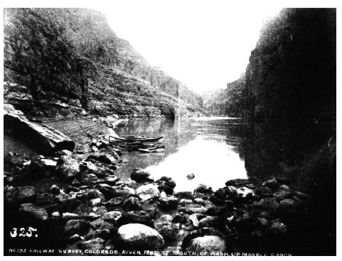
| Figure 4. Replicate photographs of the debris fan at South Canyon (river mile 32.5-R). A. Photograph taken in July 17, 1889 by Franklin A. Nims. The debris fan is relatively small, and boats were parked relatively close to the mouth of the canyon. |
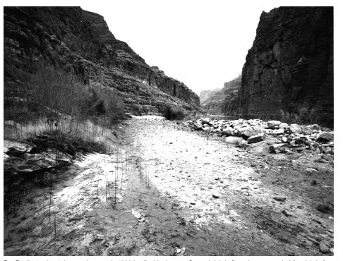 |
| Figure 4. Continued. B. Replicate view taken on January 2, 1992 by Jim Hasbargen. Several debris flows have aggraded the debris fan, including a large one that deposited the prominent levee at right between 1940 and 1965. |
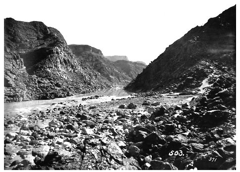 |
| Figure 5. Replicate photographs showing the debris fan at Ruby Rapid (river mile 104.8-L) (Webb, 1996). A. Photograph taken on February 15, 1890 at 1:00 PM by Robert B. Stanton. Lack of sand in the canyon mouth, and freshlooking gravels all the way to the river, indicates a flash flood had recently occurred in Ruby Canyon, probably in the summer of 1889. |
 |
|
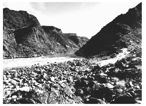
Figure 5. Continued. |
The century over which we measure the binomial frequency of debris flows is determined by a remarkable baseline of photographs taken in 1889 and 1890 by Franklin A. Nims and Robert B. Stanton (Melis and others, 1994; Webb, 1996). A total of 445 photographs record the general topography of the river corridor at roughly 2-km intervals along the entire length of Grand Canyon. We replicated the Nims and Stanton photographs between 1990 and 1994 (Webb, 1996); in addition, we used 38 photographs of the Canyon taken by John K. Hillers in 1872 (Fowler, 1989). A total of 178 of these 483 photographs capture debris fans at the confluences of 164 of the 600 tributaries and the Colorado River in Grand Canyon (fig. 6). These 164 fans form the “calibration set” of our data.
 |
| Figure 6. Histograms comparing the sample drainage-basin areas with the population drainage-basin areas of tributaries in Grand Canyon. |
One important limitation of this data set is that the photographic record captures only the mouths of the tributary canyons. Thus, binomial-frequency estimates are skewed to record only those debris flows large enough to reach the Colorado River. Therefore, we do not include all debris flows generated in tributaries, but only those that have reached the river.
We measured 21 variables representing the morphometric, lithologic, climatic and structural drainage-basin characteristics that may control or influence debris-flow initiation in Grand Canyon (table 2). These include standard drainage-basin measures such as area, channel length, and channel gradient. All three major debris-flow source lithologies (Hermit Shale, the Supai Group, and Muav Limestone) are represented by their height above river level, a measure of the potential energy of source failures. We also included the height above river level of the highest point in each drainage basin. Although this variable does not relate directly to source failures, it does reflect the potential for intense rainfall and the potential energy of runoff, which are factors in some types of failures. A large amount of initial energy may not translate into a debris flow, however, if the transit distance to the river is sufficiently long. The greater the distance, the more energy is lost in transit (Savage and Hutter, 1987), and fewer and smaller debris flows reach the river. Therefore, we also measured channel distance from each source lithology to the river. The inter-dependence of source height and channel distance from river are represented in a third class of variable, channel gradient from source area to river, a simple ratio of channel distance to source height.
| Table 2. Drainage-basin parameters used in logistic regression. | ||||
|
|
||||
| Variable | Variable name | Approximate1 probability distribution |
Range in values | Units |
|---|---|---|---|---|
|
|
||||
| Drainage-basin area | AREA | lognormal | -1.3 to 3.8 | km2 |
| Height above river of: | ||||
| - headwaters | HEADHT | normal | 402 to 2207 | m |
| - Hermit Shale | HERMHT | bimodal normal | 0 to 1488 | m |
| - Supai Group | SUPHT | bimodal normal | 0 to 1134 | m |
| - Muav Limestone | MUHT | bimodal normal | 0 to 890 | m |
| Inverse of channel length to: | ||||
| - headwaters | HEADD | lognormal | -1.8 to 0.3 | log (m)-1 |
| - Hermit Shale | HERMD | bimodal lognormal | -3.0 to 0.7 | log (m)-1 |
| - Supai Group | SUPD | bimodal lognormal | -3.0 to 1.0 | log (m)-1 |
| - Muav Limestone | MUD | bimodal lognormal | -3.0 to 1.0 | log (m)-1 |
| Channel gradient to: | ||||
| - headwaters | HEADG | lognormal | -1.8 to 0.3 | none |
| - Hermit Shale | HERMG | bimodal lognormal | -3.0 to 0.7 | none |
| - Supai Group | SUPG | bimodal lognormal | -3.0 to 0 | none |
| - Muav Limestone | MUG | bimodal lognormal | -3.0 to -0.2 | none |
| Elevation of: | ||||
| - headwaters | HEADEL | normal | 1061 to 2804 | m |
| - Hermit Shale | HERMEL | bimodal normal | 0 to 2073 | m |
| - Supai Group | SUPEL | bimodal normal | 0 to 1951 | m |
| - Muav Limestone | MUEL | bimodal normal | 0 to 1707 | m |
| Tributary aspect | TASP | uniform | 0 to 1.0 | none |
| River aspect | RASP | uniform | 0 to 1.0 | none |
| Log of total length of faults | FAULT | normal | -2 to 2.3 | log (km) |
| River kilometer | RKM | uniform | 4.5 to 395.9 | km |
|
|
||||
| 1 Bimodal normal, the distribution is normal except for zero values. Bimodal lognormal, the distribution is lognormal except for transformed zero values. | ||||
Few Grand Canyon tributaries have climatic stations, so precipitation associated with debris flows must be estimated using data collected many kilometers away. Because of this, we derived proxy variables to measure climatic effects on debris-flow initiation. Elevations of source lithologies and basin headwaters above sea level are included to reflect orographic effects on precipitation. Higher elevations are likely to intercept more moisture as precipitation and so produce more debris flows. Additionally, tributaries which open into the dominant paths of weather systems and moisture vectors may actively trap precipitation, particularly smaller storms. Tributaries facing other directions may be orographically shielded from many storms.
We calculated the aspect, F, for each drainage as the angle from true north of a ray drawn from the basin centroid to its confluence with the river. This radial measure was then transformed into a linear value more appropriate for logistic regression modeling: southwestern aspect (θ), the degree to which a given drainage faces southwest using
| θ; = sin[(Φ - 45°)/2]. , | (3) |
An orientation to the southwest was chosen to reflect the southwest to northeast travel vectors of severe weather across Grand Canyon. Similarly, we measured the aspect of the canyon or river-corridor itself as the angle from true north of a vector drawn parallel to the river at the confluence of each tributary. This value, which we termed Θ, was linearized into a variable of southwest/northeast trend in the river corridor runs using
| Θ = |cos(Φ - 45°)|. | (4) |
The influence of geologic structure in each drainage was evaluated as the linear sum of all surface faults delineated on geologic maps of the area (Haynes and Hackman, 1978; Huntoon and others, 1981; Huntoon and Billingsley, 1983; Huntoon and others, 1986). One important difficulty with these data is that geologic map coverage of the study area is not at a uniform scale: map scales ranged from 1:250,000 to 1:48,000. Thus, on the basis of scale variation alone, apparent fault density may differ from one area to another depending on the map used. In this case, fault density may increase artificially from east to west, because map scales increased in that direction.
We also included a measure of river kilometer, the distance in kilometers along the river from Lees Ferry to the confluence with each tributary. This variable is intended to reflect any ordered spatial variation in debris-flow frequency along the river corridor that is not accounted for by the other variables.
All drainage-basin data were measured from USGS 7.5’ topographic maps (1:24,000 scale) and various geologic maps (Haynes and Hackman, 1978; Huntoon and others, 1981; Huntoon and Billingsley, 1983; Huntoon and others, 1986). For source lithologies, elevations, heights above and channel distance from the river, we averaged the largest and smallest values measured to the bottom of the units. We calculated an inverse-channel distance variable, which is the reciprocal of channel distance. For lithologic strata that are not present in a given basin, zero values were entered for their variables. Gradient was calculated simply as height above river divided by channel distance, and so is also a mean value. Drainage-basin boundaries were drawn by hand on topographic maps, digitized, and entered into a GIS, which calculated drainage areas and centroids.
Because the dependent variable, debris-flow frequency, is binomial, we chose logistic regression for modeling the relation of drainage-basin variables to debris-flow frequency. Where linear regression returns a continuous value for the dependent variable, logistic regression returns the probability of a positive binomial outcome (in this case, debris-flow occurrence during the last century). Logistic regression is commonly used in medical and biological studies where the dependent variable is the presence or absence of a given illness or disease, and independent variables the presumed controlling factors. In medical research, logistic regression is used to analyze the statistical significance of certain factors in relation to diseases, as well as for modeling the probability of contracting the disease on the basis of the significant controlling factors (Hosmer and Lemeshow, 1989).
For logistic regression, the conditional mean probability, (π(x)) is:
| π(x) = eg(x) / [1 + eg(x)], | (5) |
where
| g(x)=β0 + βixi + β2x2 + ... + βixi | (6) |
and i = number of variables. The coefficients (βv) are estimated by the method of maximum likelihood, where coefficients with the highest probability of returning the observed values are selected. Maximum likelihood is determined using the likelihood function, which expresses the probability of the observed data as a function of the unknown coefficients (Hosmer and Lemeshow, 1989). Those coefficients that maximize the likelihood function are thus the coefficients with the greatest probability of returning the observed values. SAS statistical software was used to calculate these model coefficients as well as various measures of their significance (SAS, 1990). After the coefficients are estimated using the calibration set, and verified as reasonable using the verification set, we calculated the probabilities of debris-flow occurrence for all 600 tributaries using equations (5) and (6).
Our 9,516 km2 study area is too geomorphically diverse to be effectively treated in one model of Grand Canyon; drainage-basin lithology and morphology differ markedly over the length of the Colorado River. Instead, we separated the initial 164 drainages with known debris-flow frequencies into two distinct data sets, one each for eastern and western Grand Canyon. It is extremely difficult to identify a unique point of geomorphic transition between the eastern and western canyon as a variety of major structural and morphometric changes occur between Phantom Ranch (river mile 97.8) and Crystal Creek (river mile 98.2). The margin faults passing across Grand Canyon at Crystal Creek (Hunter and others, 1986) suggested that mile 98 was the approximate point of separation between eastern and western Grand Canyon. Splitting the data at river mile 98.0 (Crystal Creek) resulted in models that presented the best balance in terms of model fit and stability. Moving the point of separation east or west from this location excessively strengthened one model at the expense of the other. Separating the data at river mile 98.0 placed 78 drainages in eastern Grand Canyon (river mile 0 to 98.0) and 86 drainages in western Grand Canyon (river mile 98.1 to 248.3). These data, which we call the “calibration set,” do not represent a random sample of our population, based as they are on the historical photographic evidence available to us. Nevertheless, a comparison of the sample and population distributions of each drainage-basin variable indicates that the sample is statistically representative of the population of ungaged tributaries throughout Grand Canyon (fig. 6).
We used principal-component analysis to identify the drainage-basin variables that are statistically redundant. After a qualitative assessment of the redundant variables that contribute to the effectiveness of the model (usually on the basis of increased information content), the extraneous variables were eliminated from further consideration. Variables measuring distance or area, such as drainage area, channel distances, channel gradient, and fault distance, are distributed logarithmically. Logistic regression is not dependent on normally distributed data, but log transformation of these variables reduces the redundancy identified by principal-component analysis. We therefore chose to use the logtransformed values in modeling the probability of debris-flow occurrence. To properly evaluate zero values in log-transformed data, zero values were replaced with a value one order of magnitude smaller than the smallest non-zero variable. For source-lithology channel distances and gradients this value was 0.001, resulting in a log-transformed value of -3. For fault lengths, these values were 0.01 and -2.
We used a step-backward elimination process in our logistic regression (SAS, 1990). Variables of least statistical significance are removed from the model until only variables with significance (ρv) less than a given threshold (0.10 in this study) remain. We used the χ2 measure of the Wald statistic (Hosmer and Lemeshow, 1989; SAS, 1990) to evaluate variable significance. We employed several statistics to evaluate the quality of the resulting models. These statistics include measures of the overall significance of the final model compared with the model containing all initial variables (ρm); a percentage of accurately predicted debris-flow occurrence as a rough measure of model accuracy (α); and the Hosmer/ Lemeshow model goodness-of-fit statistic (C), which can be expressed as a χ2 significance measure (ρC) (Hosmer and Lemeshow, 1989).
We also calculated the odds ratio (Ψ) for each variable in the model. This statistic measures the change in the odds of outcome occurrence per unit increase of the variable. We evaluated how robust the models were by attempting to reproduce model results using larger data sets drawn from the same population of drainages. For this purpose, we determined debris-flow probability for the “verification set,” an additional 50 drainages—25 each in eastern and western Grand Canyon—using a variety of non-photographic methods, including radiometric dating, stratigraphic evidence, and other field evidence (Melis and others, 1994). Unfortunately, a verification set of only 25 observations is too small for reliable logistic regression modeling alone. We therefore added each set of 25 drainages to the original calibration data and formed two larger verification data sets (fig. 7). This overlap of calibration and verification data limits the usefulness of the model comparison.
 |
| Figure 7. Map of Grand Canyon showing the locations of tributaries with histories of debris flows between 1890 and 1990. |
Next: Initiation of Debris Flows
| AccessibilityFOIAPrivacyPolicies and Notices | |
 |
|