

8. Appendix - digital data at FTP site
TABLE 1. Eastern Aleutian arc 3D model layers
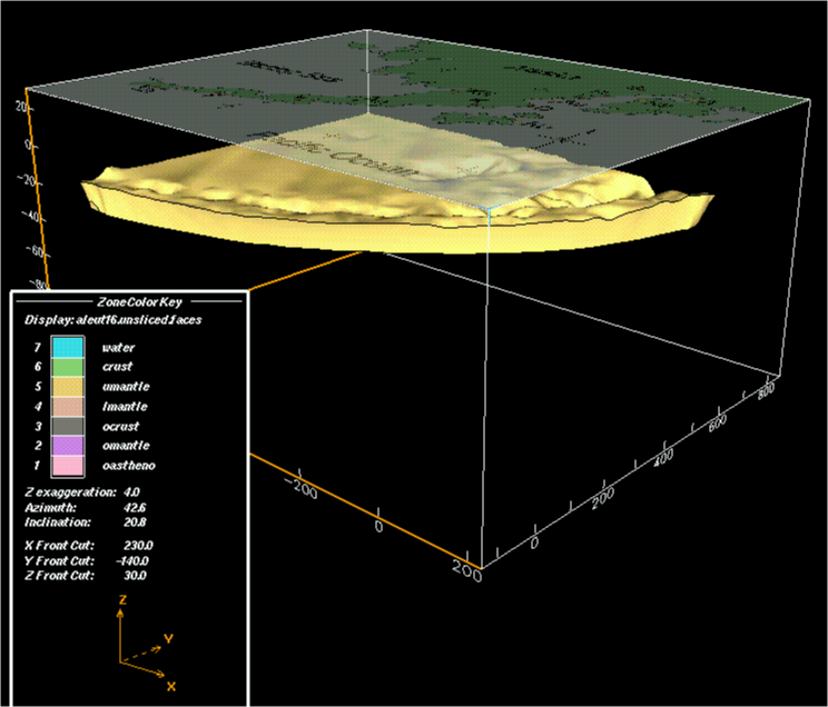
FIGURE 1. Annotated view of the eastern Aleutian volcanic arc model
FIGURE 2. World plate boundary map with location of eastern Aleutian arc.
FIGURE 3. Components of a typical ocean/continent subduction zone.
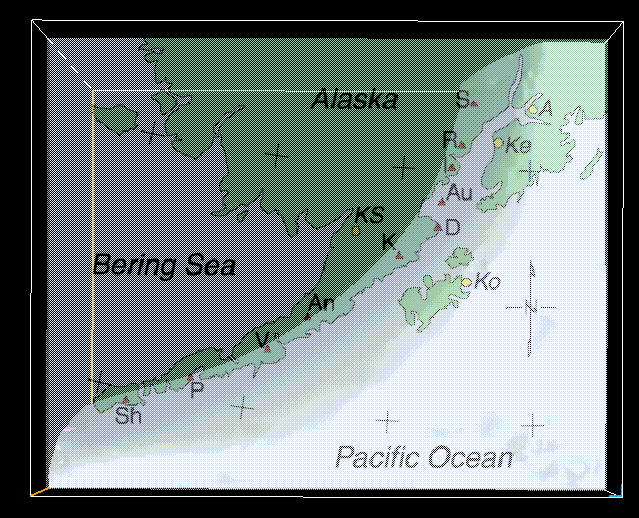
FIGURE 4. Topographic/geographic location map for the eastern Aleutian arc.
FIGURE 5. Seismic gaps along the eastern Aleutian arc.
FIGURE 6. Water layer of the eastern Aleutian arc 3D model.
FIGURE 7. Continental crust layer of the Aleutian arc 3D model.
FIGURE 8. Bathymetry/Topography data from Sandwell compilation.
FIGURE 9. Continental upper mantle layer of the Aleutian arc 3D model.
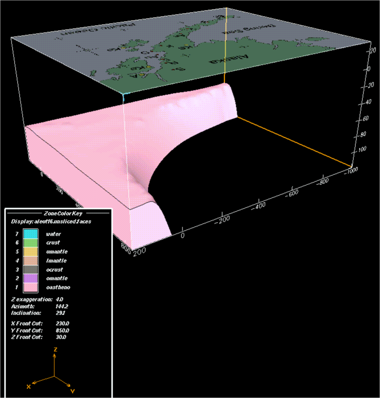
FIGURE 10. Continental asthenosphere layer of the Aleutian arc 3D model.
FIGURE 11. Oceanic crust layer of the Aleutian arc 3D model.
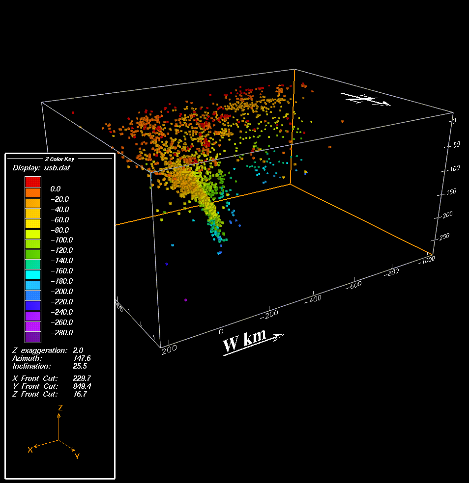
FIGURE 12. Earthquake epicenters from the CNSS catalog 1990-1999.
FIGURE 13. Oceanic mantle layer of the Aleutian arc 3D model.
FIGURE 14. Oceanic asthenosphere layer of the Aleutian arc 3D model.
FIGURE 15. Magnetic isochrons near the eastern Aleutian trench.
FIGURE 16. Oceanic lithosphere thickness verses age.
FIGURE 21. Geometry of volcanic arc relative to trench and deep slab.
FIGURE 22. Model view #1 with ocean-corrected free-air gravity draped on top.
 Click on the figure to view a full-sized version.
A 3-dimensional model (Figure 1) of the interaction of oceanic and continental tectonic plates along the eastern portion of the Aleutian volcanic arc helps in the visualization of basic tectonic, geodetic, and geophysical data in this active plate boundary region. The model is constrained by topographic, bathymetric, and seismic data and by the principle of isostasy. Examination of free-air gravity anomalies over the region indicates where the flexural strength of the down-going oceanic slab disturbs local isostatic balance and where low-density sediments have accumulated in the trench and forearc regions.
 Click on the figure to view a full-sized version.
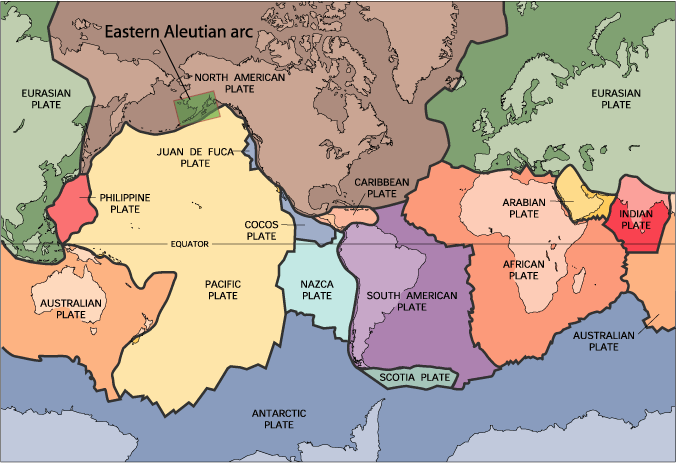
The Earth's tectonic plates (Figure 2) produce spectacular topography, active volcanoes, and powerful earthquakes when they collide at convergent boundaries. When the collision is between a continental and an oceanic plate, as in the eastern Aleutian arc, the dense, heavy oceanic plate will subduct beneath the lighter continental plate. The crust of continental plates is 25-50 km thick and predominately made of low density, silica-rich felsic rocks; oceanic plates have a crust that is 5-10 km thick and composed of dense, iron-rich mafic rocks.
 Click on the figure to view a full-sized version.
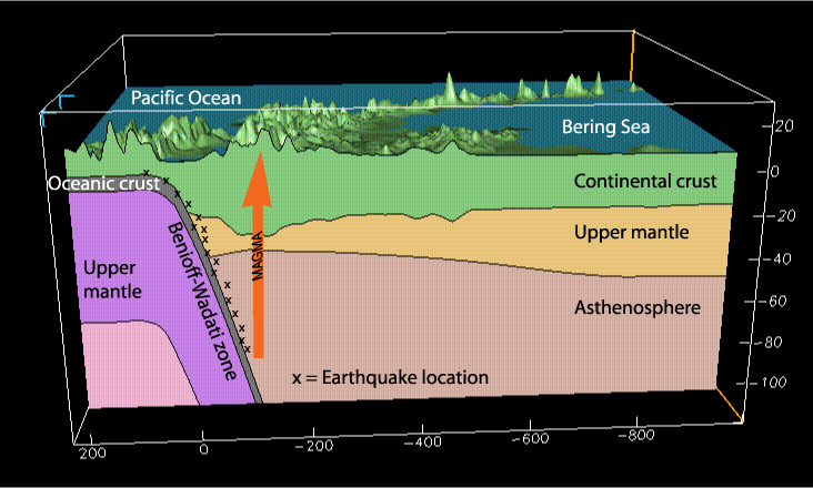
Figure 3 depicts the components of a typical subduction zone. In this diagram the oceanic plate is subducting from left to right beneath the continental plate on the right. Surficial features diagnostic of a subduction zone include the bathymetric trench formed above the point of maximum bending in the down-going plate, the accretionary wedge of sediments that accumulates in the trench region, the forearc region where the continental crust tends to be stretched and thinned and sediments may accumulate, and the volcanic arc that overlies the zone where magma is generated by the interaction of fluids from the oceanic plate with deep rocks of the overriding plate (at about 100 km depth).
Earthquakes occur as a result of stresses created in subducting one rigid tectonic plate beneath another. Near the Earth's surface, extensional type earthquakes occur in the flexural bulge formed at the point of maximum bending of the down-going plate. Compressional earthquakes tend to occur in the accretionary wedge region as sediments scraped off the downgoing plate pile up. A set of earthquakes follows the upper part of the downgoing plate and mark what is called the Wadati-Benioff zone (e.g., Lillie, 1999).
 Click on the figure to view a full-sized version.
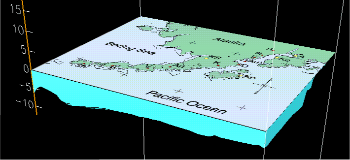
The eastern Aleutian arc extends approximately 1,000 km from Unimak Pass on the west to the vicinity of Spurr Volcano on the east (Figure 4). This seismically active region is currently monitored by three cooperating groups. The U.S. Geological Survey and the State of Alaska fund the Alaska Volcano Observatory and the Alaska Earthquake Information Center, both of which operate seismic networks. Additional stations are operated by the US West Coast and Alaska Tsunami Warning Center. The USGS National Earthquake Information Center, using data from the three local networks and from additional global stations, also locates events in this region. We used the composite earthquake catalog of the Council of the National Seismic System (CNSS) for the Aleutian arc region from 1990-1999 to trace the 3-dimensional shape of the subducting Pacific Plate.
 Click on the figure to view a full-sized version.
All the rupture zones of the eastern Aleutian arc west of Kodiak Island are considered to be seismic "gaps" (according to Nishenko and Jacob, 1990) because they have historic records of great earthquakes, yet have not experienced great earthquakes in the last 3 decades. In addition to serious damage to port and canning facilities in the sparsely populated local region, great earthquakes may generate tsunamis (tidal waves) that threaten coastal regions of the western United States and Hawaii.
We used the principle of isostasy to hypothesize a plausible shape for the base of the continental crust in this 3D model. Isostasy is a concept that explains the inverse correlation between topography and Bouguer gravity anomalies. Under the Airy model for local isostasy (Airy, 1855; Simpson and others, 1986), the crust is assumed to be composed of uniform density material that floats on a higher-density material (the mantle). Thus the base of the crust is an exaggerated reflection of the topography, similar to the base of lower-density icebergs floating on higher-density water (Lillie, 1999). As depicted in our models, mountainous areas reveal the most dramatic effects of isostasy. In order to support the weight of mountains, the crust must have thicker roots, which mirror the mountains above the surface.
Of course the real crust/mantle boundary (called the Moho or Mohorovic discontinuity) is defined as the boundary between Earth layers with differing seismic velocities (the speed that very low frequency sound waves travel through the ground) and is not necessarily a big density contrast. There is also no requirement that crustal density loads be isostatically in balance in an actively subducting region. Still, the isostatic model provides a way of visualizing the amount of buoyancy required to support the spectacular topography of the region. We expect that the actual Moho probably lies within 5 km of our predicted Moho and follows the same general shape. Our model could be greatly improved by detailed analysis of teleseismic data (the seismograph records of far away earthquakes whose seismic energy passes through this region) and local active source seismic surveys.
To establish a plausible thickness for the Pacific plate along this part of the Aleutian arc, we used the relationship between ocean lithosphere thickness and age (e.g., Leeds and others, 1974; Turcotte and Schubert, 1982). Oceanic plates are formed at mid ocean ridges, where hot mantle flows upward to the surface. Through time, as the newly formed oceanic lithosphere moves further from the ridge, the lithosphere cools and thickens.
The geologic model for the eastern Aleutian arc has the following layers:
| Table 1. Eastern Aleutian arc 3D model layers | |
|---|---|
| Name | Description |
| water | Sea water - top at sea level. |
| crust | Continental crust - top defined by topography and bathymetry. |
| umantle | Continental upper mantle - top defined by isostatic Moho. |
| lmantle | Continental asthenosphere - top defined as an upwarping surface beneath the volcanic arc. |
| ocrust | Oceanic crust - top defined by bathymetry and by earthquake epicenters. |
| omantle | Oceanic mantle - top defined by depth offset from top of subducting slab. |
| oastheno | Oceanic asthenosphere - top defined by depth offset from the top of the oceanic mantle. |
In order to depict east-west and north-south map dimensions in true relative scale we have used an Albers conformal map projection to convert latitude and longitude coordinates to kilometers on the ground. The parameters of the projection are: standard parallels = 55°, 65° central meridian = -151°, base latitude = 55° datum = Clark, 1866. The x axes of our figures thus represent kilometers in the west to east direction and the x values range from -1000 to 230 (zero falls at the central meridian of the projection, 151° west longitude). The y axes of our figures represent kilometers in the south to north direction and range from -140 to 850 (zero falls at the base latitude of the projection, 55° north latitude). For detailed information on map projections, consult Snyder (1983).
Two different models, with differing vertical scales and ranges were constructed. Model 1 has a vertical scale that ranges from -120 to +30 km. For model 1 the vertical scale above sea level is exaggerated by 10 times compared with the vertical scale below sea level. Thus, the +30 km model elevation represents +3 km in real-world elevation. Model 2 has no changes in vertical elevation scale and ranges from -25 to +3 km.
 Click on the figure to view a full-sized version.
The water layer is simply defined as a geologic layer with the top at zero elevation. This layer overlies the crust and ocrust layers where they lie below sea level.
 Click on the figure to view a full-sized version.
 Click on the figure to view a full-sized version.
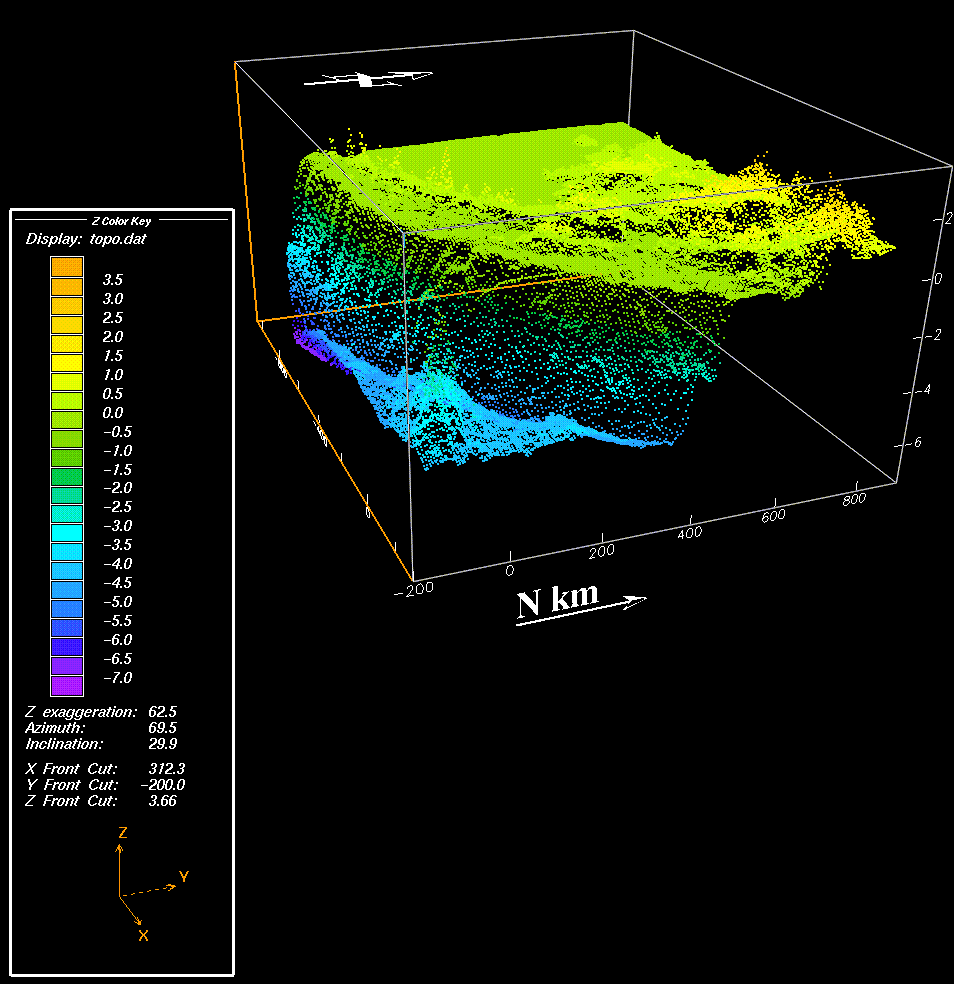
The continental crust layer (Figure 7) has a top defined by bathymetric and topographic data (Figure 8). The bathymetry data are derived from satellite altimetry (Sandwell and Smith, 1997). The digital topography in the Sandwell compilation is based on the GTOPO30 digital elevation model.
 Click on the figure to view a full-sized version.
The continental upper mantle layer (Figure 9) has a top defined by the shape of buoyant crustal roots required to isostatically support topography. For our isostatic model we assumed that continental crust is 25 km thick when its top lies at sea level, that the density contrast between the light crust and heavy upper mantle is 0.35 g/cc, and that rocks above sea level have an average density of 2.67 g/cc. As discussed in the introduction section above, this is an idealized model of the actual crust/mantle boundary and could easily be off by 5 km from an actual seismic measurement of the Moho at any given point.
 Click on the figure to view a full-sized version.
The contental asthenosphere layer (Figure 10) has a top defined as a gently upwarping surface starting at 60 km depth and shallowing to about 40 km depth beneath the volcanic arc. This shape for the asthenosphere is based a written communication from Chris Nye, University of Alaska Fairbanks. Modern models of the deep Earth structure at volcanic arcs generally include a shallowing of the asthenosphere beneath the volcanic axis.
 Click on the figure to view a full-sized version.
 Click on the figure to view a full-sized version.
The oceanic crust layer (Figure 11) has a top defined by bathymetry (Figure 8) and the upper boundary of deep seismicity (Figure 12). The seismicity data consist of 3149 epicentral solutions taken from the Composite Earthquake Catalog Archive of the Council of the National Seismic System (CNSS) . Typical magnitudes range from 3 to 5 MW. Depths range from 3 km above sea level to 270 km below sea level, with a mean depth of about 70 km. The dates of the earthquakes range from 1/4/1990 to 7/4/1999. The data are compiled from several sources, including the Alaska Earthquake Information Center located at the University of Alaska, Fairbanks, and the U.S. Geological Survey National Earthquake Information Center located in Golden, Colorado.
 Click on the figure to view a full-sized version.
The oceanic mantle layer (Figure 13) has a top defined as a 7 km constant thickness beneath the top of the oceanic crust. This represents the typical worldwide average thickness of oceanic crust (i.e., Turcotte and Schubert, 1982).
 Click on the figure to view a full-sized version.
 Click on the figure to view a full-sized version.
 Click on the figure to view a full-sized version.
The oceanic asthenosphere (Figure 14) layer has a top defined as a constant 70 km thickness beneath the top of the oceanic crust. This thickness was chosen by comparing the average age of the oceanic lithosphere at the eastern Aleutian trench (Figure 15) with a worldwide plot of age verses thickness for oceanic lithosphere (Figure 16; Turcotte and Schubert, 1982). Careful mapping of the magnetic stripes (Severinghaus and Atwater, 1990) caused by remanent magnetization of the oceanic crust indicate that the age of the oceanic lithosphere ranges from about 50 million years to about 55 million years from east to west across the eastern Aleutian trench (Figure 15). This corresponds (Figure 16) to a total expected lithosphere thickness of about 70 km.
The previous sections show views of each layer of the model and explain the basic data that constrained the shape of these layers. This section briefly describes some lessons we learned in building the 3D model using the EarthVision software package. Some of these lessons and limitations will quickly become dated because of the rapid pace at which the capability of hardware and software increases.
When constructing a 3D model it is important to realize that you have to provide data that will constrain the shape of each model interface over the entire lateral extent of your model space. It is generally unsatisfactory to count on gridding algorithms to fill out portions of your model that lack data. We found that we had to pay particular attention to the corners of our model; we constructed data points by hand, when necessary, that were centered right in the middle of the corner cells of our model to ensure that corners of layers didn't dip up or down precipitously.
We were unable to find a way to automatically create a layer with a constant thickness below or above a fixed interface (as required for our oceanic mantle and asthenosphere tops) within EarthVision. The EarthVision option for a constant thickness layer makes a layer with a constant depth offset. This, of course, only works with a layer with a flat reference surface, otherwise the layer thickness will vary as a function of slope of the reference surface. We wrote a FORTRAN program, gdthicklayer, that inputs a gridded surface and outputs scattered x,y,z data points that define a surface with a constant thickness offset from the gridded surface. The source code for this program is provided in the FTP area of this report.
It appears to us that current memory and cpu speed constraints limit the size of workable EarthVision 3D models to a pixel cube with about 100 elements in each dimension. This limitation prevents use of the full resolution of some data sets, such as detailed digital elevation models, in construction of regional geologic models such as ours.
 Click on the figure to view a full-sized version.
 Click on the figure to view a full-sized version.
In these views (Figures 17 and 18) we are looking to the southwest down the Aleutian peninsula. The deep part of the model has a four times vertical exaggeration relative to the lateral distance scales. In addition, the topography has been vertically exaggerated by ten times relative to the depth scale below sea level. The purpose of this vertical exaggeration is to allow simultaneous viewing of topographic details as well as deep subduction zone structure.
In Figure 17 the water, crust, ocrust, and lmantle layers are all shown as solid bodies. The umantle, omantle, and oastheno layers are depicted as transparent. Figure 18 is similar except that the water layer has also been made transparent so that the location of the trench can be seen and the omantle layer is solid to depict the full down-going slab.
Note the arcuate form of the volcanic chain located inboard of the bend in the downgoing plate. Also note how the isostatic Moho (base of the crust layer) mirrors topography. This long-wavelength mirror image effect is accentuated by the vertical exaggeration of topography in this model view.
 Click on the figure to view a full-sized version.
This view is looking to the northwest up the Aleutian chain toward Cook Inlet. The vertical exaggeration is the same as the preceeding view. All layers above the ocrust layer are depicted as transparent. This includes the water, crust, umantle, and lmantle layers. This display allows examination of the relative position of the volcanic arc with the bend in the down-going slab.
 Click on the figure to view a full-sized version.
In this view (looking to the northeast), the vertical exaggeration of topography relative to the deeper portions of the model has been turned off. Note that the overall vertical scale is still exaggerated by ten times relative to the lateral scales, however. The water layer is transparent to allow viewing of the trench where the ocrust and crust layers intersect. The omantle layer is also transparent in this view.
 Click on the figure to view a full-sized version.
Note the position of the volcanic chain above the curved line formed by the intersection of the downgoing slab with a depth of 100 km.
 Click on the figure to view a full-sized version.
This is a southwest view of the model (same perspective as Figure 17) with "ocean-corrected" free-air gravity anomalies painted onto the top surface of the model. To produce the gravity image we started with free-air gravity data from Sandwell and Smith (1997). We then used the top and bottom of the water layer to calculate the three-dimensional effect of the low-density water on free-air gravity using the Simpson implementation (Robert Simpson, USGS, written communication, 1991) of the Parker method (Parker, 1972).
The ocean-corrected free-air gravity anomaly shows a long-wavelength, trench-parallel high with two superimposed, shorter-wavelength, trench-parallel lows. The overall broad, long-wavelength gravity high is probably caused by the local isostatic imbalance that results from flexural upwarping of the subducting plate. The flexural strength of the oceanic slab causes the topographic loads above this part of the subduction zone to be supported without the need for low density roots directly beneath the loads. The lack of these low density roots relative to adjacent regions results in the long-wavelength gravity high.
Superimposed on this broad gravity high are two trench-parallel lows. The outboard and most pervasive of the gravity lows occurs directly over the trench itself and is probably caused by the accumulation of low-density sediments in the accretionary wedge filling the bathymetric depression of the trench. Moving inboard, the second trench-parallel gravity low occurs just outboard of the volcanic arc, extending from the Cook Inlet in the north, through the Shelikof Strait, and terminating at Stepovak Bay. This low probably represents thick accumulations of continental sediments in the forearc basin. Detailed modeling of these gravity features, partularly in conjunction with constraints from seismic reflection and refraction data, could be used to determine structural details of these sedimentary rock accumulations.
Readily available regional datasets, such as earthquake catalogs, digital elevation models, and satellite gravity models, combined with commercial three-dimensional modeling and visualization software, allow the construction of simple three-dimensional models of regional tectonic features. Our simple model of the eastern Aleutian volcanic arc permits visualization of the spatial relationship of the trench, subducting slab, and volcanic arc.
Initial analysis of free-air gravity data over the eastern Aleutian arc shows a regional, trench-parallel high, probably caused by isostatic "undercompensation" of the flexurally supported bending bulge of the subducting plate. This regional high is striped by two trench-parallel lows, probably caused by low-density sediments accumulated in the trench and in the Cook Inlet to Stepovak Bay forearc basin region.
Airy, G.B., 1855, On the computation of the effect of the attraction of the mountain-masses, as disturbing the apparent astronomical latitude of stations in geodetic surveys: Philisophical Transactions of the Royal Society of London, v. 145, p. 101-104.
Ernst, W.G., 1990, The Dynamic Planet: Columbia University Press, NewYork, 281 pp.
Leeds, A.R., Knopoff, L., and Kausel, E.G., 1974, Variations of upper mantle structure under the Pacific Ocean: Science, v. 186, p. 141-143.
Lillie, R.J., 1999, Whole Earth Geophysics: An Introductory Textbook for Geologists and Geophysicists: Prentice Hall, New Jersey, 361 pp.
Nishenko, S.P., and Jacob, K.H., 1990, Seismic Potential of the Queen Charlotte-Alaska-Aleutian seismic zone: Journal of Geophysical Research, v. 95, n. B3, p. 2,511-2,532.
Parker, R.L., 1972, The rapid calculation of potential anomalies: Geophysical Journal of the Royal Astronomical Society, v. 31, p. 447-455.
Sandwell, D.T., and Smith, W.H.F., 1997, Marine Gravity Anomaly from Geosat and ERS-1 Satellite Altimetry: Journal of Geophysical Research, v. 102, n. B5, p. 10,039-10,054.
Snyder, J.P., 1983, Map projections used by the U.S. Geological Survey: U.S. Geological Survey Bulletin B1532, 313 pp.
Turcotte, D.L. and Schubert, G., 1982, Geodynamics: Applications of Continuum Physics to Geological Problems: John Wiley & Sons, NewYork, 450 pp.
Severinghaus, J. and Atwater, T., 1990, Cenozoic Geometry and Thermal State of the Subducting Slabs Beneath Western North America: in, Wernicke, B.P. (ed.), Basin and Range Extensional Tectonics Near the Latitude of Las Vegas, Nevada, Geological Society of America Memoir 176, p. 1-22.
Simpson, R.W., Jachens, R.C., Blakely, R.J., and Saltus, R.W., 1986, A new isostatic residual gravity map of the conterminous United States with a discussion on the significance of isostatic residual anomalies: Journal of Geophysical Research, v. 91, p. 8,348-8,372.
The FTP site contains a FORTRAN program (source code), digital data files, and VRML (virtual reality meta language) versions of the Aleutian volcanic arc model. VRML files may be viewed interactively using freely available web browser plug-ins (see, for example, the VRML repository).
The following digital files and data are available via FTP:
1. gdthicklayer.f - a FORTRAN program to calculate the position
                    of a surface that is offset by a constant
                    thickness from an input grid surface.

2. model1a.wrl.gz - a VRML (virtual reality meta-language) version of
                  the eastern Aleutian volcanic arc model.  The file is
                  compressed using the gzip protocol.

3. model1b.wrl.gz - another VRML version of the eastern Aleutian volcanic
                  arc model.  The file is compressed using the gzip protocol.

4. crust.dat - ASCII file containing points that define the top surface
               of the crust layer (no vertical exaggeration).  Data columns
               are X, Y, Z with all coordinates in kilometers.

5. crustx10.dat - ASCII file containint points that define the top surface
                  of the crust layer (with 10 times vertical exaggeration).
                  Data columns are X, Y, Z with all coordinates in kilometers.

6. moho.dat - ASCII file containing points that define the top surface
                 of the umantle layer.  Data columns are X, Y, Z in km.

7. astheno.dat - ASCII file containing points that define the top surface
                  of the astheno layer.  Data columns are X, Y, Z in km.

8. ocrust.dat - ASCII file containing points that define the top surface
                of the ocrust layer.  Data columns are X, Y, Z in km.

9. omantle.dat - ASCII file containing points that define the top surface
                 of the omantle layer.  Data columns are X, Y, Z in km.

10. oastheno.dat - ASCII file containing points that define the top surface
                  of the oastheno layer.  Data columns are X, Y, Z in km.

11. eq.pdat - Earthquake data used to constrain the top of the ocrust layer.
              Data columns are X, Y, Z, eq magnitude.

12. topo.dat - Topography/bathymetry data used to constrain the top of the
               ocrust and crust layers.  Data columns are X, Y, Z in km.
Saltus, R.W., and Barnett, A., 2000, Eastern Aleutian Volcanic Arc Digital Model - Version 1.0: U.S. Geological Survey Open-File Report 00
-365.
| AccessibilityFOIAPrivacyPolicies and Notices | |
| |
|