METHODS

Benthic habitat and geologic mapping were conducted with combined interferometric side-scanning sonar and video-camera sled onboard the research vessel R/V Shearwater from August 8 to August 27, 2005 (The cruise report can be viewed online at http://walrus.wr.usgs.gov/infobank/s/s105sc/html/s-1-05-sc.meta.html).

Sonar Data

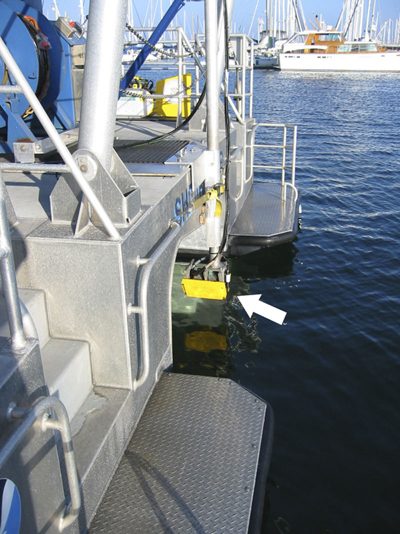
Interferometric sonar data were collected using a 468 kHz SEA Swathplus Interferometric sonar. Interferometric sonar imaging provides high-resolution images of the sea floor by recording the intensity of sound reflected off the sea floor (acoustic backscatter). In addition seafloor depth data are estimated from the phase difference between seafloor reflections received by spaced receivers. The sonar was mounted on a pole manufactured expressly for use on the R/V Shearwater.

Figure 2. Custom mount for the interferometric sonar on the R/V Shearwater fantail.  Pole can be raised using wire from small winch running through a block on the A-frame. The arrow points to the Interferometric sonar head. For a larger view, click the above image.

Top of Page

Sea Floor Video

Video imagery of the sea floor in the area mapped with sonar at depths of 20-70 m was obtained on the final 3 days of the USGS research cruise aboard the R/V Shearwater.

The techniques used to characterize the video observations real-time on the boat were consistent with methods described by Anderson et. al. (in press). The objectives of seafloor video characterization were to: (1) record geologic and biologic characteristics of the seafloor real-time, (2) ground-truth geophysical data (bathymetry and backscatter) by resolving both common and unique features of the sea floor, and (3) examine regions of transition between different substrate types as suggested in acoustic backscatter data. Video observations were subsequently used to construct maps of substrate type and habitat distribution and to provide a measure of uncertainty in the final products. Thus, video transect locations were selected on the basis of the existence, quality, and complexity of sonar data and on regions of geologic transition and/or biologic significance.

The underwater video sled (Fig. 3) was towed behind the vessel, and the winch operator maintained its altitude above the seafloor at 1-7 m as much as possible. The R/V Shearwater was generally drifting during video transects, because the coastal currents were adequate to transport the boat at speeds over 1 knot. Video footage was recorded to digital mini-DV tape and then copied to DVD. Ship position was determined by a CSI Wireless differential geographic positioning system (dGPS). All instrument data were multiplexed through a sub-sea housing and transmitted by the 12-conductor cable to a topside console. Latitude, longitude, height above the seafloor, pitch, roll, water depth, ship speed, ship heading, and Greenwich Mean Time (GMT) were continuously imprinted on the digital video tape while recording. These data were also automatically recorded once per every 10 seconds in a navigational text file. Positional accuracy of the sled relative to the ship's dGPS position varied with water depth, current speed and direction, and environmental conditions. Cable layback was not measured directly but was estimated to be approximately equal to the water depth during most deployments

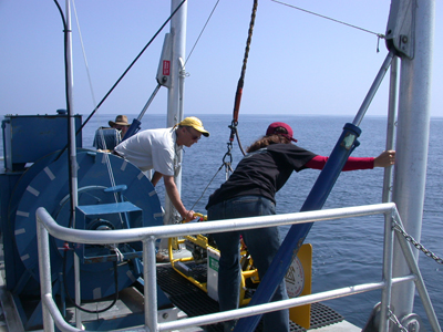
Figure 3. Sam Johnson, WCMG Team Chief Scientist, and Nadine Golden, GIS Specialist, assist the launch of the camera sled. Mike Boyle, Marine Electronics Technician, controls the A-frame and winch that lift and launch the camera sled off the back deck of the R/V Shearwater.

Top of Page

Sea floor characteristics were observed and recorded digitally real-time at 30 second intervals by a geologist and a biologist watching the towed video. Observations included geomorphology, sediment texture, and biota, and observation codes were entered as comments in YoNav navigation software (Gann, 1992) using an "X-Keys" programmable keypad and a Dell Inspiron 8100 laptop computer. Time (GMT), dGPS position, and other ship data for were automatically recorded in the text file each time an observation event was entered. Observations at each event included:

• primary and secondary substrate type (e.g. boulder/cobble, rock/sand, mud/mud)
• substrate complexity (rugosity)
• seafloor slope
• benthic biocoverage (low, medium, or high)
• the presence of benthic organisms and demersal fish
• small-scale sea-floor features (e.g., ripples, tracks, and burrows).

The resulting product from the video observations is the point shapefile "video_observations." Each point includes the date, latitude/longitude location, depth, primary and secondary substrate, observer comments, and the absence of presence of the following biota and physical characteristics: algae, anemone, bivalve, brittle start, crustacean, cup coral, driftweed, fishing gear, fishing trash, flatfish, gastropod, gorgonian, hole, hydrozoa, interface, kelp, mound, octopus, other fish, rockfish, rubble, scour, sea cucumber, sear hare, sea pen, sea star, sea whip, sediment ripple, sediment wave, sheep head, sponge, tracks, tube worm, and urchin.

Nearly 14 hours of both vertical and oblique underwater video were collected and logged real-time in this manner on 14 transects of the coast of Santa Barbara, in Southern California (view a location map of video observations).

Data Processing

Seafloor observations and geophysical data were co-registered, integrated, and analyzed using the following data processing methods. Navigation and motion & tide correction & the backscatter intensity data were processed using SEA SwathProcessor v2.01. The data output from SEA SwathProcessor was exported in grid format and mosaicked into a continuous image of the study area using ESRI's ArcGIS v9.1. All grid calculations were performed using Python, Surfer, and ArcGIS (commands and code are available in the metadata file for each grid). The georeferenced acoustic backscatter data layer is an image built from data with a horizontal resolution of 1 m with grayscale values proportional to the acoustic backscatter intensity of the sea floor. Depth data were processed using the Python program "Bathy_proc.py." Details about depth data processing can be found in the metadata of the bathymetry raster file. The sonar data set covers 77 square km and is divided into 125 lines. Detailed processing steps performed on ach of these 125 lines were:

Processing backscatter sonar lines

• Imported each raw backscatter line into “SonarWiz.MAP.”
• Used “SonarWiz.MAP Sonar File Manager” tool to check and correct the navigation data
• Manually “bottom-tracked” each line
• Applied signal processing functions by setting the Automatic Gain Control (AGC), Beam Angle Correction (BAC), project sonar data using sensor headings
• Individually exported each line as a GeoTif file.
• Used Python program to loop through the directory of GeoTif files and convert GeoTif to ArcGIS raster format
• Removed “NoData” raster cells using the ArcGIS Con statement; and projected the data to WGS 1984 UTM Zone 11.
• In ArcGIS, imported lines according to track line number
• Mosaiced adjacent backscatter lines and masked lines to remove far range data, and not average overlapping data. 

Processing bathymetry data

• Based on the Julian date at original data collection, chronologically imported each raw bathymetry file into “SEA Swath Processor Real-Time Software System.”
• Configured the way the data was processed in “SEA Swath Processor” by inputting adjustment and offset information, such as ship's motion, tides, velocity of sound, and relative sensor positions.
• Monitored the data once through in real-time and noted the ping numbers where data needed adjustments.
• Saved data by re-running the line and made corrections at problematic ping numbers by adjusting the bathymetric filters accordingly to improve the quality of the processed data.
• Used Python script, “Bathy_proc.py” designed to filter the bathymetry text file and then convert the bathy data to ArcGIS raster format.
• In ArcGIS, imported lines according to track line number. Mosaiced adjacent bathymetry lines masked lines to remove far range data, and not average overlapping data.

Top of Page

Analytical Methods for Seafloor Classification

Interpretation of the processed sonar data and video observations resulted in predictions of benthic habitat distribution in the region. These predictions are distinguished as habitat classification codes that follow the "Deep-Water Marine Benthic Habitat Classification Scheme; Key to Habitat Classification Code for Mapping and use with GIS programs." (modified after Greene et al., 1999). The Deep-Water Marine Benthic Habitat Classification process and scheme is outlined below.

Generating habitat polygons

• The area mapped by sonar was classified using the “Supervised Maximum Likelihood Classification” tool of the Spatial Analyst extension in ESRI ArcGIS 9.1.
• Seven data layers were coregistered in an ESRI ArcMap Project:
  1. euclidean distance (ESRI, 2005) grid of track lines.
  2. mosaiced backscatter at 2 meter resolution
  3. entropy from backscatter (Cochrane and Lafferty, 200) at 2 meter resolution
  4. homogeneity of backscatter (Cochrane and Lafferty, 200)at 2 meter resolution
  5. rugosity derived from mosaiced bathy using the Benthic Terrain Modeling Tool’s Rugosity Builder (Lundblad et al., 2006).
  6. enthropy from backscatter (Cochrane and Lafferty, 200) at half meter resolution
  7. homogeneity of backscatter (Cochrane and Lafferty, 200) at half meter resolution
• Supervisory signatures were designed by using video observations and then were generated using the above seven layers and ESRI’s ArcGIS Create signatures tool.
• Three Greene et al. (1999) bottom induration classes were output and the output three class grid was converted to polygons using ArcGIS Grid to Polygons Conversion tool.
• The resulting polygons were further subdivided based on seafloor slope, complexity, and bathymetric depth. The additional Greene et al. (1999) attributes Meso/Macrohabitat and Modifier were added based on proximity to video observations. A detailed description of the process steps can be found in the “All Habitat” Shapefile metadata.
• Used select by attribute, location, and manual selection tools to query and assign Green habitat code attributes. Decreased number of polygon attributes by grouping polygons of like classification if polygons area less or equal to 10 sq meters.

The Greene et al. (1999) habitat code attribute list is outlined below.

Top of Page

Mega Habitat

Megahabitat - Use capital letters (based on depth and general physiographic boundaries; depth ranges approximate and specific to study area).

A = Aprons, continental rise, deep fans and bajadas (3000-5000 m)

B = Basin floors, Borderland types (floors at 1000-2500 m)

F = Flanks, continental slope, basin/island-atoll flanks (200-3000 m)

I = Inland seas, fiords (0-200 m)

P = Plains, abyssal (>5000 m)

R = Ridges, banks and seamounts (crests at 200-2500 m)

S = Shelf, continental and island shelves (0-200 m)

Seafloor Induration

Seafloor Induration - Use lower-case letters (based on substrate hardness).

h = hard bottom, rock outcrop, relic beach rock or sediment pavement

m = mixed (hard & soft bottom)

s = soft bottom, sediment covered

Sediment types (for above indurations) - Use parentheses.

(b) = boulder

(c) = cobble

(g) = gravel

(h) = halimeda sediment, carbonate

(m) = mud, silt, clay

(p) = pebble

(q) = shell hash

(s) = sand

Top of Page

Meso/Macrohabitats

Meso/Macrohabitat - Use lower-case letters.

a = atoll

b = beach, relic

c = canyon

d = deformed, tilted and folded bedrock

e = exposure, bedrock

f = flats

g = gully, channel

i = ice-formed feature or deposit, moraine, drop-stone depression

k = karst, solution pit, sink

l = landslide

m = mound, depression

n = enclosed waters, lagoon

o = overbank deposit (levee)

p = pinnacle

r = rill

s = scarp, cliff, fault or slump

t = terrace

v = depression (flat bassin)

w = sediment waves

x = nearshore

y = delta, fan

z_# = zooxanthellae hosting structure, carbonate reef

1 = barrier reef

2 = fringing reef

3 = head, bommie

4 = patch reef

Top of Page

Modifier

Modifier - Use lower-case subscript letters or underscore for GIS programs (textural and lithologic relationship).

_a = anthropogenic (artificial reef/breakwall/shipwreck)

_b = bimodal (conglomeratic, mixed [includes gravel, cobbles and pebbles])

_c = consolidated sediment (includes claystone, mudstone, siltstone, sandstone, breccia, or conglomerate)

_d = differentially eroded

_f= fracture, joints-faulted

_fb = any mass of fish, squid or aggregating species that reflects sonar

_g = granite

_h = hummocky, irregular relief

_i = interface, lithologic contact

_k = kelp

_l = limestone or carbonate

_m = massive

_p = pavement

_r = ripples

_s = scour (current or ice, direction noted)

_t = heavily bioturbated

_u = unconsolidated sediment

_v = volcanic rock

Top of Page

Seafloor Slope

Seafloor Slope - Use category numbers. Calculated for survey area from x-y-z multibeam data.

1 = Flat (0-1º)

2 = Sloping (1-30º)

3 = Steeply Sloping (30-60º)

4 = Vertical (60-90º)

5 = Overhang (> 90º)

Seafloor Complexity

Seafloor Complexity - Use category letters (in caps). Calculated for survey area from x-y-z multibeam slope data using neighborhood statistics and reported in standard deviation units.

A = Very Low Complexity (-1 to 0)

B = Low Complexity (0 to 1)

C = Moderate Complexity (1 to 2)

D = High Complexity (2 to 3)

E = Very High Complexity (3+)

Seafloor Depth

Seafloor Depth - Use category numbers enclosed by curly brackets. Calculated for survey area from x-y-z multibeam data.

{1} Intertidal

{2} Intertidal to 30m

{3} 30m to 100m

{4} 100m to 200m

{5} 200m and deeper)

Top of Page