Click on figures for larger images.

Figure 1. Map showing locations where long- and short-term shoreline change rates were calculated based on extent of available shoreline data in Washington.

Figure 2. Map showing locations where long- and short-term shoreline change rates were calculated based on extent of available shoreline data in Oregon.

Figure 3. Example of an end point rate calculation using a sample dataset. The rate of 1.09 meters per year is calculated as the distance between the shorelines in 1936 (baseline) and 2005 (76.03 meters) and divided by the span of time elapsed between the two shoreline positions (69.82 years). All other shoreline data are ignored in this computation. Figure from Himmelstoss (2009).

Figure 4. Example of a linear regression rate calculation using a sample dataset. The shoreline change rate was determined by plotting the shoreline positions with respect to time and calculating the linear regression equation of y = 1.34x – 2,587.4. The slope of the equation describing the line is the rate (1.34 meters per year) in this example. Figure from Himmelstoss (2009).

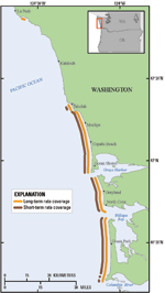
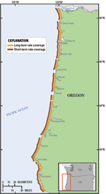
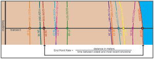
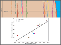
This section describes the methods used to compile shoreline data and calculate rates-of-change for the Pacific Northwest Coast.

Shoreline Data

Historical shoreline data were acquired from multiple sources and have been documented in the shoreline attribute table and metadata files in this report. Shoreline data were digitized from National Oceanographic and Atmospheric Administration (NOAA) topographic sheets (T-sheets) and aerial photographs. The dates of historical shorelines range from 1868 to 1999. A modern shoreline derived from lidar topographic surveys is from data collected in 2002. The lidar data were collected by the USGS in collaboration with the National Aeronautics and Space Administration (NASA). Data used in this study are part of the 2002 Airborne Lidar Assessment of Coastal Erosion (ALACE) Project for California, Oregon, and Washington coastlines. Index maps showing data coverage are displayed (figs. 1 and 2).

The historical shorelines are based on an interpreted high water line (HWL) that was digitized from topographic maps and aerial photographs. The shorelines extracted from lidar data are referenced to mean high water (MHW), an elevation datum-based shoreline that is different from the HWL, a proxy-based physical feature shoreline. The HWL shorelines are consistently landward of the MHW shorelines, and the offset between the datum- and proxy-based shorelines can be considered a bias (Ruggiero and others, 2003). This bias value varies alongshore and is documented in an accessory table associated with the lidar shoreline. Bias values were used in the rate calculation process to reconcile the offsets between the HWL and MHW shorelines. All distance measurements are referenced to MHW before rate calculation.

Lidar data were not available for all sandy beaches along the Pacific Northwest coast; gaps exist mainly in northern Washington.

Additional information regarding the shoreline compilation methods, measurement uncertainties, and a summary of the results can be found in (Ruggiero and others, 2013).

Calculation of Shoreline Change Rates

Rates of shoreline change were generated within Esri ArcMap version 9.3 using the Digital Shoreline Analysis System (DSAS) version 4.2, an Esri ArcGIS tool developed by the USGS (Thieler and others, 2009). The tool is a freely available application designed to work within the ArcGIS software. The DSAS was used to generate orthogonal transects starting from a reference baseline and intersecting the shoreline positions at 50-meter intervals. The distance measurements between the transect and shoreline intersections and the baseline were then used to calculate the rate-of-change statistics. A linear regression method was used to calculate rates of change over the long term (about 100 years), and an end point rate calculation was used to capture potential changes in trends or rates over the short term (about 30 years).

End Point Rates (Short-Term)

Short-term rates of shoreline change were calculated for each transect using an end point rate calculation between the shoreline position from the 1980s (Washington) or 1967 (Oregon) and the modern, lidar-derived shoreline (2002) to provide an approximate 20- or 30-year short-term rate. The end point rate is calculated by subtracting the difference in shoreline position between the two survey years and dividing it by the time between surveys to give a rate in meters per year (fig. 3). The end point rate was not assumed to be linear between the two survey years; this rate simply represents the net change between the two shorelines, annualized to facilitate comparisons with long-term rates found through linear regression. The short-term transect metadata files provide descriptions of the two fields associated with the end point rate calculation. The end point confidence interval, which is not currently included in the DSAS version 4.2 software, was computed using a customized module compatible with DSAS. The confidence interval of the end point rate calculation is described in detail within the short-term transect metadata files. Additional information on the end point rate calculation can be found in section 7 of the DSAS user guide.

Linear Regression Rates (Long-Term)

Long-term rates of shoreline change, in meters per year, were calculated at each transect as the slope of the linear regression through all shoreline positions from the earliest (1800s) to the most recent (the 2002 lidar-derived shoreline). Data for a minimum of four available shoreline-survey years (one of which must be the lidar-derived shoreline) were required at each DSAS transect for calculating long-term rates. The linear regression method of determining shoreline-change rates was based on an assumed linear trend of change between the earliest and latest shoreline dates (fig. 4). Data for shoreline areas where such a linear trend did not exist and shoreline-change rates have not remained constant through time would produce a poor linear fit to the data with a higher reported uncertainty. The long-term transect metadata files provide descriptions of the four fields associated with the linear regression rate calculation, and additional information can be found in section 7 of the DSAS User Guide.

To view files in PDF format, download a free copy of Adobe Reader.