Click on figures for larger images.

Figure 1. Index map of the Massachusetts coast showing the 10 geographic regions used to organize and publish the shoreline rate-of-change data in this report.

Figure 2. Map illustrating the extent of shoreline coverage for Massachusetts. Yellow lines represent historic shoreline data referenced to the high water line. Red lines represent lidar-extracted shoreline positions referenced to the mean high water line.

Figure 3. Example of a linear regression shoreline change rate calculation using a sample dataset. The rate was determined by plotting the shoreline positions with respect to time and calculating the linear regression equation of y = 1.34x – 2587.4. The slope of the equation describing the line is the rate (1.34 m/yr). Figure from Himmelstoss (2009).

Figure 4. Example of an end point rate calculation using a sample dataset. The rate of 1.09 meters per year is the distance between the 2005 and 1936 shorelines (76.03 meters) divided by the span of time elapsed between the two shoreline positions (69.82 years). All other shoreline data are ignored in this computation. Figure from Himmelstoss (2009).

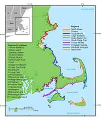
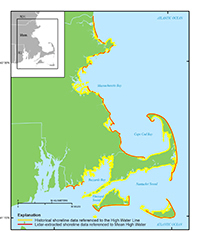
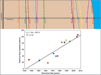
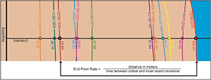
This section describes the methods used to compile shoreline data and calculate rates of change for the Massachusetts Shoreline Change Project. Two different vertical datums are used to reference the water level position of the shorelines based on the data source used to interpret the location. The historical shorelines derived from NOAA T-sheets and orthophotographs are proxy-based and referenced to the high water line (HWL). Shorelines derived using lidar data are tidal-based and referenced to the mean high water (MHW) position. The HWL shorelines are consistently landward of the MHW shorelines and the offset between the two positions is a consistent proxy-datum bias (Ruggiero and List, 2009). These proxy-datum bias values change for each geographic region and are determined during the process of extracting a shoreline position from the lidar data. The bias values are stored in several uncertainty tables associated with the originally- published lidar data (See Geospatial Data section). These values are incorporated into the analysis performed by the Digital Shoreline Analysis System (DSAS) software, which reconciled the offsets between the HWL and MHW shorelines before computing rate-of-change results (See appendix 2 of the DSAS user-guide for a more detailed explanation). Lidar data were not available for the entire Massachusetts coast; gaps exist within the regions (fig.1) of Boston, Cape Cod Bay, South Cape Cod, the Elizabeth Islands, and Buzzards Bay (fig. 2). When shorelines within these regions were uniformly referenced only to the HWL the proxy-datum bias correction was not necessary. Further details describing the methods, measurement uncertainties and a summary of the results are documented in the Massachusetts Shoreline Change Mapping and Analysis Project, 2013 Update (Thieler and others, 2013).

Calculation of Shoreline Change Rates

Rates of shoreline change were calculated using the DSAS version 4.3; an ArcGIS tool developed by the USGS (Thieler and others, 2009). DSAS is a freely-available application designed to work within the Esri ArcGIS software. A reference baseline was constructed offshore from the time series of shorelines and was positioned to conform to changes in the combined orientation of the shorelines alongshore. DSAS was used to generate orthogonal transects at 50-m spacing along the coast starting from the reference baseline and intersecting the shoreline positions. The distance measurements (meters) along every transect from the reference baseline to each shoreline intersection were used to calculate the rate-of-change statistics. A linear regression method was used to calculate long-term (approximately100 year) rates of change. Short-term (approximately 30 year) rates were calculated using the linear regression method if enough data was available (more than 3 shorelines), otherwise the end-point rate method was used.

Long-Term Rates (1800s to 2009)

Long-term rates of shoreline change, in meters per year, were calculated at each transect by finding the slope of the best-fit line through all shoreline positions from the earliest (1800s) to the most recent (2008, 2009, or the 2007 lidar-derived shoreline). Long-term rates also were calculated without shorelines (at a request of the CZM) from the 1970s (from the years 1970 to 1972, 1975, 1978, 1979) and 1994 to examine the potential impact of including or excluding these data on the measured rates of change. When calculating linear regression rates, a minimum of three available shoreline survey years were required at each DSAS transect. The linear regression method of determining shoreline change rates assumes a linear trend of change between the earliest and most recent shoreline dates (fig. 3). In areas where a linear trend does not exist and shoreline positions have not progressed uniformly in one direction through time, it is expected that the resulting linear fit to the data will be poorer, and the linear regression rate will have a higher reported uncertainty. The metadata for the long-term transect shapefiles provide descriptions of the four attribute fields associated with the linear regression rate calculations. Additional information can be found in the Massachusetts Shoreline Change Mapping and Analysis Project, 2013 Update (Thieler and others, 2013) or section 7 of the DSAS user guide (Himmelstoss, 2009).

Short-Term Rates (1970–1982, 1994 to 2008/2009)

Short-term rates of change were calculated at each transect for the more recent 30 years of shoreline data (beginning between 1970–1982 and ending with data from 1994, 2008 or 2009) using the linear regression method. In addition, short-term end-point rates were calculated at any transect that had only two shorelines available within this time period. The Boston and the Elizabeth Islands geographical regions lacked shoreline position data prior to 1994, so end-point rates for those regions were calculated for a 14- or 15-year interval (1994 to 2008 or 2009). The end-point rate is calculated by taking the difference in shoreline position between the two dates and dividing that by the duration of time between surveys to report a rate in meters per year (fig. 4). The end-point rate simply represents the net change between the surveys, annualized to facilitate comparisons with long-term linear regression rates. The short-term transect metadata files provide descriptions of the attribute field associated with the end-point rate calculation. Additional information can be found in the Massachusetts Shoreline Change Mapping and Analysis Project, 2013 Update (Thieler and others, 2013) or the DSAS user guide (Himmelstoss, 2009).