Professional Paper 1722
In cooperation with the Wisconsin Department of Natural Resources
1 U.S. Geological Survey, Wisconsin Water Science Center, Middleton,
Wisconsin
2 Wisconsin Department of Natural Resources, Monona, Wisconsin
3 Michigan
Department of Natural Resources, Ann Arbor, Michigan
4 Wisconsin
Department of Natural Resources, Madison, Wisconsin
Purpose and Scope
Approach
Methods of Data Collection and Analysis
Field Methods
Watershed Boundaries and Environmental Characteristics
Data Summaries
Statistical Methods
Water Quality and Its Relations with Environmental Characteristics in the Watershed
Relations between Water Quality and Environmental Characteristics in the Watershed
Regionalization Schemes for Reference Water Quality and the Response in Water Quality to Changes in Land Use
Relations with Individual CharacteristicsMacroinvertebrate Communities and Their Relations with Water-Quality, Environmental, and Physical-Habitat Characteristics
Effects of Multiple Characteristics on Benthic Chlorophyll a Concentrations and Diatom Indices
Reference Values for Benthic Chlorophyll a Concentrations and Diatom Indices
Relations with Individual CharacteristicsFish Communities and Their Relations with Water-Quality, Environmental, and Physical-Habitat Characteristics
Effects of Multiple Characteristics on Macroinvertebrate Indices
Reference Values for the Macroinvertebrate Indices
Relations with Individual Characteristics
Effects of Multiple Characteristics on Fish Indices
Reference Values for the Fish Indices
Multiparameter Biotic Indices to Estimate Nutrient Concentrations in Wadeable Streams
Final Regionalization Scheme for Wisconsin Streams
Reference Conditions
Responses of Water Quality to Changes in Land Use
Responses of Biotic Indices to Changes in Nutrient Concentrations
Multiparameter Biotic Indices to Estimate Nutrient Concentrations in Wadeable Streams
Nutrient Concentrations Controlling the Biotic Integrity of Streams
Appendix 1. Stream identification information, location information, and summary statistics for flow and water-quality data collected for each of the 240 studied wadeable streams in Wisconsin.
Appendix 2. Physical-habitat characteristics of each of the 240 studied wadeable streams in Wisconsin.
Appendix 3. Diatom nutrient-tolerance ranking for individual diatom taxa.
Appendix 4. Biological data for each of the 240 studied wadeable streams in Wisconsin.
Figure 1. National nutrient ecoregions and major land uses in the upper Midwest.
Figure 2. Two regionalization schemes considered for wadeable streams in Wisconsin: A, level III ecoregions with major land-use/land-cover categories and B, environmental phosphorus zones.
Figure 3. Environmental phosphorus zones in the upper Midwest.
Figure 4. Sites on wadeable streams in Wisconsin included in this study.
Figure 5. Distributions of median monthly total phosphorus, total nitrogen, and suspended chlorophyll a concentrations, and Secchi tube depth.
Figure 6. Total phosphorus and total nitrogen concentrations as a function of the percentage of total agriculture in the watersheds of the studied wadeable streams in Wisconsin.
Figure 7. Suspended chlorophyll a concentrations and Secchi tube depths as a function of median total phosphorus and total nitrogen concentrations.
Figure 8. Percentages of explained variance in water quality described by anthropogenic/land-use, basin, soil and surficial-deposit characteristics, and interactions among categories.
Figure 9. Percentages of explained variance in A, Secchi tube depths and B, suspended chlorophyll a concentrations described by nutrients, environmental characteristics, and interactions among categories.
Figure 10. Percentiles of A, total agriculture in the watersheds, B, total phosphorus, and C, total nitrogen in streams in the level III ecoregions and environmental phosphorus zones.
Figure 11. A, suspended chlorophyll a concentrations and B, Secchi tube depths in Reference sites, High sites, and sites with only reference total nitrogen or reference total phosphorus concentrations.
Figure 12. Total phosphorus concentrations as a function of the percentage of agricultural land use in A, environmental phosphorus zones and B, level III ecoregions, and response curves for phosphorus concentrations as a function of the percentage of agriculture in the watershed, in C, EPZs, and D, level III ecoregions.
Figure 13. Total nitrogen concentrations as a function of the percentage of agricultural land use in A, environmental phosphorus zones and B, level III ecoregions, and response curves for nitrogen concentrations as a function of the percentage of agriculture in the watershed, in C, EPZs, and D, level III ecoregions.
Figure 14. Suspended chlorophyll a concentrations as a function of total phosphorus and total nitrogen concentration, by environmental phosphorus zones and by level III ecoregions.
Figure 15. Secchi tube depth as a function of total phosphorus and total nitrogen concentration, by environmental phosphorus zones and by level III ecoregions.
Figure 16. Response curves for A, suspended chlorophyll a concentrations and B, Secchi tube depths in the environmental phosphorus zones as a function of the percentage of agriculture in the watershed.
Figure 17. Distributions of benthic chlorophyll a concentrations, Diatom Nutrient Index values, Diatom Siltation Index values, and Diatom Biotic Index values.
Figure 18. Benthic chlorophyll a concentrations, Diatom Nutrient Index values, and Diatom Siltation Index values as a function of total phosphorus and total nitrogen concentration in the environmental phosphorus zones and level III ecoregions.
Figure 19. Benthic chlorophyll a concentrations, Diatom Nutrient Index values, and Diatom Siltation Index values as a function of dissolved phosphorus, dissolved nitrite plus nitrate, dissolved ammonia, and total Kjeldahl nitrogen concentrations in the environmental phosphorus zones.
Figure 20. Benthic chlorophyll a concentrations and Diatom Nutrient Index values for five nutrient categories.
Figure 21. Percentage of explained variance in benthic chlorophyll a concentrations and diatom index values described by nutrients, other water-quality characteristics, environmental and physical-habitat characteristics, and interactions among categories.
Figure 22. Benthic chlorophyll a concentrations, Diatom Nutrient Index, Diatom Siltation Index, and Diatom Biotic Index values in Reference sites, High sites, and sites with only reference total nitrogen or reference total phosphorus concentrations.
Figure 23. Distributions of macroinvertebrate Hilsenhoff Biotic Index values, the percentages of individuals that were Ephemeroptera, Plecoptera, or Trichoptera, and the percentages of taxa that were Ephemeroptera, Plecoptera, or Trichoptera.
Figure 24. Hilsenhoff Biotic Index values, the percentages of individuals that were Ephemeroptera, Plecoptera, or Trichoptera, and the percentages of taxa that were Ephemeroptera, Plecoptera, or Trichoptera as a function of total phosphorus and total nitrogen concentration in the environmental phosphorus zones and level III ecoregions.
Figure 25. Hilsenhoff Biotic Index values, the percentages of individuals that were Ephemeroptera, Plecoptera, or Trichoptera, and the percentages of taxa that were Ephemeroptera, Plecoptera, or Trichoptera as a function of dissolved phosphorus, dissolved nitrite plus nitrate, dissolved ammonia, and total Kjeldahl nitrogen concentrations in the environmental phosphorus zones.
Figure 26. Percentages of explained variance in six macroinvertebrate index values described by nutrients, other water-quality characteristics, environmental and physical-habitat characteristics, and interactions among categories.
Figure 27. Hilsenhoff Biotic Index values, the percentages of individuals that were Ephemeroptera, Plecoptera, or Trichoptera, and the percentages of taxa that were Ephemeroptera, Plecoptera, or Trichoptera in Reference sites, High sites, and sites with only reference total nitrogen or reference total phosphorus concentrations.
Figure 28. Distributions of fish Index of Biotic Integrity values, the percentages of the fish that are carnivorous, the percentages of fish considered pollution intolerant, and the number of fish caught.
Figure 29. Fish Index of Biotic Integrity values, the percentages of fish considered pollution intolerant, and the percentages of the fish that are carnivorous as a function of total phosphorus and total nitrogen concentration in the environmental phosphorus zones and level III ecoregions.
Figure 30. Fish Index of Biotic Integrity values, the percentages of fish considered pollution intolerant, and the percentages of the fish that are carnivorous as a function of dissolved phosphorus, dissolved nitrite plus nitrate, dissolved ammonia, and total Kjeldahl nitrogen concentrations in the environmental phosphorus zones.
Figure 31. Percentages of explained variance in eight fish index values described by nutrients, other water-quality characteristics, environmental and physical-habitat characteristics, and interactions among categories.
Figure 32. Fish Index of Biotic Integrity values, the percentages of the fish that are carnivorous, and the percentages of fish that are considered pollution intolerant in Reference sites, High sites, and sites with only reference total nitrogen or reference total phosphorus concentrations.
Figure 33. Measured and estimated A, total phosphorus and B, total nitrogen concentrations for the four-parameter regression models, C, measured phosphorus concentrations as a function of Biotic Index of total Phosphorus values, and D, measured nitrogen concentrations as a function of Biotic Index of total Nitrogen values.
Figure 34. Proposed regionalization scheme for defining nutrient criteria for wadeable streams in Wisconsin.
Table 1. Reference concentrations for total phosphorus, total nitrogen, and suspended chlorophyll a, and turbidity in selected national nutrient and level III ecoregions and environmental phosphorus zones.
Table 2. Summary statistics for median monthly water-quality and environmental characteristics of the watersheds of the sites in the studied wadeable streams in Wisconsin.
Table 3. Median and average monthly concentrations for total and dissolved phosphorus, suspended chlorophyll a, total nitrogen, nitrite plus nitrate, ammonia, and Kjeldahl nitrogen, and Secchi tube depths.
Table 4. Spearman correlation coefficients between median concentrations of total phosphorus, dissolved phosphorus, total nitrogen, nitrite plus nitrate, ammonia, total Kjeldahl nitrogen, median Secchi tube depths, suspended chlorophyll a concentrations, percentages of urban and agricultural areas, point-source loadings of phosphorus, and specific environmental characteristics.
Table 5. Spearman correlation coefficients between residualized logarithmically transformed median concentrations of total phosphorus, dissolved phosphorus, nitrogen, nitrite plus nitrate, total Kjeldahl nitrogen, ammonia and suspended chlorophyll a, median Secchi tube depths, and specific residualized environmental characteristics.
Table 6. Results of forward stepwise-regression analyses used to explain the variance in raw and residualized water-quality concentrations.
Table 7. Results from redundancy analysis between water-quality and environmental characteristics.
Table 8. Reference conditions for total phosphorus, total nitrogen, and suspended chlorophyll a concentrations, and Secchi tube depths in the environmental phosphorus zones and level III ecoregions.
Table 9. Responses in total phosphorus total nitrogen, suspended chlorophyll a, and Secchi tube depth to changes in the percentage of agricultural land use in the watershed.
Table 10. Summary statistics for the physical-habitat characteristics and biotic indices.
Table 11. Spearman rank correlation coefficients between benthic chlorophyll a concentrations and diatom community indices, and median water-quality, environmental, and physical-habitat characteristics.
Table 12. Thresholds or breakpoints in the responses of benthic chlorophyll a concentrations and diatom indices to changes in nutrient concentrations.
Table 13. Percentiles of total phosphorus and total nitrogen concentrations for the studied streams having both benthic chlorophyll a and diatom index data.
Table 14. Results of forward stepwise-regression analysis to explain the variance in benthic chlorophyll a concentrations and the three diatom indices.
Table 15. Spearman rank correlation coefficients between macroinvertebrate-community indices and median water-quality, environmental, and physical-habitat characteristics.
Table 16. Thresholds or breakpoints in the responses in macroinvertebrate indices to changes in nutrient concentrations.
Table 17. Results of forward stepwise-regression analyses to explain variance in macroinvertebrate indices.
Table 18. Spearman rank correlation coefficients (rs) between fish-community indices and median water-quality, environmental, and physical-habitat characteristics.
Table 19. Thresholds or breakpoints in the responses in fish indices to changes in nutrient concentrations.
Table 20. Results of forward stepwise-regression analyses to explain variance in fish indices.
Table 21. Results of forward stepwise-regression analyses to explain variance in total phosphorus and total nitrogen concentrations with biotic indices.
Table 22. Reference conditions for water quality, chlorophyll a, diatoms, macroinvertebrates, and fish indices.
Table 23. Summary of thresholds or breakpoints in the responses of suspended chlorophyll a concentrations, Secchi tube depth, and various biotic indices to changes in nutrient concentrations.
|
|
|
|
| micrometer (µm) | 0.00003927 | inch (in.) |
| millimeter (mm) | 0.03937 | inch (in.) |
| centimeter (cm) | 0.3937 | inch (in.) |
| meter (m) | 3.281 | foot (ft) |
| kilometer (km) | 0.6214 | mile (mi) |
| square meter (m2) | 0.0002471 | acre |
| square centimeter (cm2) | 0.001076 | square foot (ft2) |
| square meter (m2) | 10.76 | square foot (ft2) |
| square centimeter (cm2) | 0.1550 | square inch (in2) |
| square kilometer (km2) | 0.3861 | square mile (mi2) |
| liter (L) | 0.2642 | gallon (gal) |
| cubic centimeter (cm3) | 0.06102 | cubic inch (in3) |
| cubic meter (m3) | 35.31 | cubic foot (ft3) |
| cubic meter per second (m3/s) | 70.07 | acre-foot per day (acre-ft/d) |
| cubic meter per second per square kilometer [(m3/s)/km2] | 91.49 | cubic foot per second per square mile [(ft3/s)/mi2] |
| meter per second (m/s) | 3.281 | feet per second (ft/s) |
| millimeter per hour (mm/hr) | 0.03937 | inch per hour (in/hr) |
| millimeter per year (mm/yr) | 0.03937 | inch per year (in/yr) |
| gram (g) | 0.03527 | ounce, avoirdupois (oz) |
| kilogram (kg) | 2.205 | pound, avoirdupois (lb) |
| kilogram per square kilometer (kg/km2) | 5.70992 | pound per square mile (lb/mi2) |
| milligram (mg) | 0.00003527 | ounce, avoirdupois (oz) |
| milligram per square meter (mg/m2) | 0.000003277 | ounce, avoirdupois, per square foot (oz/ft2) |
| meter per kilometer (m/km) | 5.27983 | foot per mile (ft/mi) |
Temperature in degrees Celsius (°C) may be converted to degrees Fahrenheit (°F) as follows:
°F=(1.8x°C)+32
Specific conductance is given in microsiemens per centimeter at 25 degrees Celsius (µS/cm at 25°C).
Concentrations of chemical constituents in water are given either in milligrams per liter (mg/L) or micrograms per liter (µg/L).
| Ag | Agricultural land |
| BCHL | Benthic chlorophyll a |
| BIN | Biotic Index of total Nitrogen |
| BIP | Biotic Index of total Phosphorus |
| CARN% | Percentage of fish that are top carnivores |
| DBI | Diatom Biotic Index |
| DEM | Digital Elevation Model |
| DFA | Driftless Area level III ecoregion |
| DNI | Diatom Nutrient Index |
| DP | Dissolved phosphorus |
| DSI | Diatom Siltation Index |
| EPT | Ephemeroptera, Plecoptera, or Trichoptera |
| EPTN% | Percentage of macroinvertebrate individuals that were EPT |
| EPTTX% | Percentage of macroinvertebrate taxa that were EPT |
| EPZ | Environmental phosphorus zone |
| EV | Explained Variance |
| FISHN | Number of fish caught |
| FISHSPEC | Number of fish species caught |
| GIS | Geographic Information System |
| HBI | Hilsenhoff Biotic Index |
| High Sites | Sites with nutrient concentration above the upper 95-percent confidence limits for reference nutrient concentrations |
| IBI | Fish Index of Biotic Integrity |
| INSECT% | Percentage of fish that are insectivores |
| INTOL% | Percentage of fish that are pollution intolerant |
| Log | Logarithmic transformation to base 10 |
| n | number |
| N | Nitrogen |
| NCHF | North Central Hardwood Forest level III ecoregion |
| NLF | Northern Lakes and Forests level III ecoregion |
| NH4-N | Dissolved ammonia |
| NO3-N | Dissolved nitrite plus nitrate |
| NWIS | National Water Information System |
| OEPA | Ohio Environmental Protection Agency |
| OMNI% | Percentage of fish that are omnivorous |
| p | Probability |
| P | Phosphorus |
| PtS | Point-source loadings of phosphorus |
| r | Pearson correlation coefficient |
| rs | Spearman correlation coefficient |
| R2 | Coefficient of determination |
| Ref Sites | Sites with nutrient concentration below median reference concentrations |
| Res | Residualized |
| RDA | Redundancy analysis |
| SCHL | Suspended chlorophyll a |
| SCRAP% | Percentage of macroinvertebrates that are scrapers |
| SD | Secchi tube depth |
| SHRED% | Percentage of macroinvertebrates that are shredders |
| SPARTA | Spatial regression-tree analysis |
| SWTP | Southeastern Wisconsin Till Plains level III ecoregion |
| t | tolerance-index value |
| TAXAN | Number of macoinvertebrate taxa |
| TKN | Total Kjeldahl nitrogen |
| TOL% | Percentage of fish that a pollution tolerant |
| Urb | Urban land |
| USEPA | U.S. Environmental Protection Agency |
| USGS | U.S. Geological Survey |
| WDNR | Wisconsin Department of Natural Resources |
| < | Less than |
| % | Percentage of |
| # | Number |
Excessive nutrient (phosphorus and nitrogen) loss from watersheds is frequently associated with degraded water quality in streams. To reduce this loss, agricultural performance standards and regulations for croplands and livestock operations are being proposed by various States. In addition, the U.S. Environmental Protection Agency is establishing regionally based nutrient criteria that can be refined by each State to determine whether actions are needed to improve a stream's water quality. More confidence in the environmental benefits of the proposed performance standards and nutrient criteria will be possible with a better understanding of the biotic responses to a range of nutrient concentrations in different environmental settings.
The U.S. Geological Survey and the Wisconsin Department of Natural Resources collected data from 240 wadeable streams throughout Wisconsin to: 1) describe how nutrient concentrations and biotic-community structure vary throughout the State; 2) determine which environmental characteristics are most strongly related to the distribution of nutrient concentrations; 3) determine reference water-quality and biotic conditions for different areas of the State; 4) determine how the biotic community of streams in different areas of the State respond to changes in nutrient concentrations; 5) determine the best regionalization scheme to describe the patterns in reference conditions and the responses in water quality and the biotic community; and 6) develop new indices to estimate nutrient concentrations in streams from a combination of biotic indices. The ultimate goal of this study is to provide the information needed to guide the development of regionally based nutrient criteria for Wisconsin streams.
For total nitrogen (N) and suspended chlorophyll (SCHL) concentrations and water clarity, regional variability in reference conditions and in the responses in water quality to changes in land use are best described by subdividing wadeable streams into two categories: streams in areas with high clay-content soils (Environmental Phosphorus Zone 3, EPZ 3) and streams throughout the rest of the State. The regional variability in the response in total phosphorus (P) concentrations is also best described by subdividing the streams into these two categories; however, little consistent variability was found in reference P concentrations in streams throughout the State.
Reference P concentrations are smilar throughout the State (0.03–0.04 mg/L). Reference N concentrations are divided into two categories: 0.6–0.7 mg/L in all streams except those in areas with high clay-content soils, where 0.4 mg/L is more appropriate. Reference SCHL concentrations are divided into two categories: 1.2–1.7 µg/L in all streams except those in areas with high clay-content soils, where 1.0 µg/L may be more appropriate. Reference water clarity is divided into two categories: streams in areas with high clay-content soils with a lower reference water clarity (Secchi tube depth, SD, of about 110 cm) and streams throughout the rest of the State (SD greater than or equal to about 115 cm). For each category of the biotic community (SCHL and benthic chlorophyll a concentrations (BCHL), periphytic diatoms, macroinvertebrates, and fish), a few biotic indices were more related to differences in nutrient concentrations than were others. For each of the indices more strongly related to nutrient concentrations, reference conditions were obtained by determining values corresponding to the worst 75th percentile value from a subset of minimally impacted streams (streams having reference nutrient concentrations).
By examining the biotic community in streams having either reference P or N concentrations but not both, the relative importance of these two nutrients was determined. For SCHL, P was the more important limiting nutrient; however, for BCHL and all macroinvertebrate indices, it appears that N was the more important nutrient when concentrations were near reference concentrations. For other diatom indices and all fish indices, small additions of P or N appear to have little effect on these communities when nutrient concentrations are near reference conditions.
Concentrations of P and N in streams increase as the percentage of agricultural land increases. Concentrations of P increase more quickly and concentrations of N increase more slowly in response to increasing percentages of agriculture in areas with high clay-content soils than do streams in the rest of the State. The response in water clarity is similar in streams throughout the State; however, the streams in areas with high clay-content soils have poorer reference water clarity, and, therefore, as the percentage of agriculture increases, their clarity remains lower than in streams in areas with other soil types.
As nutrient concentrations increase, many biotic indices change. This result indicates that these nutrients have direct or indirect effects on the composition of the biotic community. Thresholds were identified at which a small change in nutrient concentrations results in a relatively large change in the biotic communities. The thresholds in the response to changes in P concentrations range from about 0.04 mg/L for BCHL, to 0.06–0.07 mg/L for diatom and fish indices, to about 0.09 mg/L for macroinvertebrate indices. The thresholds in the response to changes in N concentrations range from 0.5 mg/L for the fish indices and one macroinvertebrate index to about 0.9–1.2 mg/L for the diatom and other macroinvertebrate indices. Most of the biotic indices had a wedge-shaped response to increases in nutrient concentrations. At relatively low nutrient concentrations, the biotic indices ranged widely, but at relatively high concentrations, the indices generally were poor. The wedge-shaped distribution indicates that at low nutrient concentrations, factors other than nutrients often limit the health of biotic communities, whereas, at high nutrient concentrations, nutrients and factors correlated with high nutrient concentrations are the predominant factors.
The biotic communities that are present in a stream reflect the overall ecological integrity; therefore, they integrate the effects of many different stressors and thus provide a broad measure of their aggregate effect. Nutrient concentrations by themselves explained from about 6 to 13 percent of the total variance in the components of the biotic communities or from about 14 to 23 percent of the explained variance. Nutrient concentrations were most important in affecting SCHL concentrations and macroinvertebrate communities, and least important in affecting BCHL, periphytic diatoms, and fish-community structure. For each component of the biotic community, nutrients by themselves only explained a small part of the overall variance; about half of the variance could not be explained by the variables examined in this study and about one-third of the explained variance could not be assigned to single categories of environmental characteristics.
By use of a combination of four biotic indices, two new multiparameter indices (Biotic Index of total Phosphorus, BIP, and Biotic Index of total Nitrogen, BIN) were developed to estimate P and N concentrations in streams from biotic data collected in streams. These multiparameter models estimated high and low nutrient concentrations equally well. The BIP predicted P concentrations better than the BIN predicted N concentrations. The difference in the accuracy of these indices was consistent with biotic indices being more correlated with P concentrations than with N concentrations. This result suggests that P is more important than N in affecting most biotic communities as nutrient concentrations increase above reference concentrations.
Although specific mechanisms of how nutrients affect the biota in wadeable streams were not examined in this study, the results indicate that nutrients are important in controlling the biotic health of streams. Although the biotic-community structure represents the overall ecological integrity of the stream, nutrients alone explained only a small part of the variance in the biotic community. Therefore, it is difficult to predict the exact result of reducing nutrient concentrations without also modifying the factors typically associated with high nutrient concentrations. Nutrient concentrations in many streams, especially those in agricultural areas, are well above the concentrations where thresholds in the response were found to occur; therefore, small reductions in nutrient concentrations in these streams are not expected to have large effects on the biotic community. Even with these limitations, however, it is expected that reducing nutrient concentrations will improve the biotic community, further the beneficial ecological functioning of most streams, and improve the quality of downstream nutrient-limited receiving waters.
Elevated nutrient concentrations above background conditions are one of the most common stressors (contaminants) affecting streams throughout the United States. Problems associated with elevated nutrient concentrations in surface water are not new, but they are among the most persistent. According to the National Water Quality Inventory: 1996 Report to Congress by the U.S. Environmental Protection Agency (USEPA), 50 States, Tribes, and other jurisdictions surveyed water-quality conditions in 19 percent of the Nation's 3.6 million miles of rivers and streams and found overenrichment of nutrients to be the second most common reason for impairment following the combined effects of suspended sediment and siltation (U.S. Environmental Protection Agency, 1996). Excessive nutrients in rivers and streams can result in the overgrowth of benthic algae in shallow areas and in areas with fast current and an overabundance of phytoplankton and macrophytes in deep areas with slow current. High algal and macrophyte biomass can cause severe diurnal fluctuations in dissolved oxygen and pH because of biotic production and respiration, and can generate harmful organic materials when part of the population dies (Welch and others, 1992). These conditions can lead to an increase in the availability of toxic substances, reduction in available aquatic habitat, modifications to the composition of the biotic communities, and a decrease in the overall usefulness of the stream (Miltner and Rankin, 1998; Dodds and Welch, 2000). Excessive transport of nutrients has also been linked to eutrophication of downstream lakes and impoundments, outbreaks of Pfiesteria in bays and estuaries in various Gulf and Mid-Atlantic States, and hypoxia in the Gulf of Mexico (U.S. Environmental Protection Agency, 2000a).
Under recommendations of the Clean Water Action Plan released in 1998, the USEPA has developed a National strategy to develop waterbody-specific nutrient criteria for lakes and reservoirs, rivers and streams, wetlands, and estuaries (U.S. Environmental Protection Agency, 1998); this study is concerned with those for rivers and streams. The intent of this strategy is to get all States and tribes to establish nutrient standards, that, if enforced, will reduce nutrient concentrations and improve the beneficial ecological uses of surface waters. The best way to control nutrient concentrations is to reduce that part contributed by humans, not that part contributed naturally. It has been recognized that various environmental characteristics, such as land use, geology, soils, climate, and hydrology (including human modifications and hydrologic structures) are important in determining water quality (Monteith and Sonzogni, 1981; Clesceri and others, 1986; and Robertson, 1997). Because these characteristics vary greatly across the United States, the establishment of regional nutrient criteria makes scientific sense.
Various frameworks have been used to divide large areas into smaller areas of relatively similar environmental characteristics to minimize the natural variation in water quality within the areas and maximize the differences among the areas. One such framework is the ecoregion delineation developed and refined by Omernik (1987; 1995) and Omernik and others (2000). Ecoregions are a mapped-classification system of regions with assumed relative homogeneity in ecological characteristics. These regions were said to be defined on the basis of relative differences in a suite of environmental characteristics, such as land use/land cover, land-surface form, geology, physiography, climate, soils, potential natural vegetation, and other environmental characteristics (Omernik, 1987 and 1995). The USEPA has taken the initial step in developing regional nutrient criteria based on combining Omernik's 84 level III ecoregions into 14 national nutrient ecoregions for the conterminous United States (U.S. Environmental Protection Agency, 1998; fig. 1). On a subregional basis, such as a specific State, each of these 14 nutrient ecoregions can be further subdivided into the original level III ecoregions. Wisconsin is subdivided into two national nutrient ecoregions (ecoregions 7 and 8; fig. 1), which are further subdivided into four primary level III ecoregions: Northern Lakes and Forests (NLF), North Central Hardwood Forests (NCHF), Southeastern Wisconsin Till Plains (SWTP), and the Driftless Area (DFA)(Omernik and others, 2000; fig. 2A). In addition, there are small pieces of the Western Cornbelt Plains and the Central Cornbelt Plains ecoregions. Because the Cornbelt Plains ecoregions represent only a small part of the State, they will not be discussed in this report. The nutrient ecoregions provide an initial classification scheme for developing nutrient criteria; however, the USEPA expects individual States and tribes to evaluate and possibly develop alternative regionalization schemes (U.S. Environmental Protection Agency, 2000b).
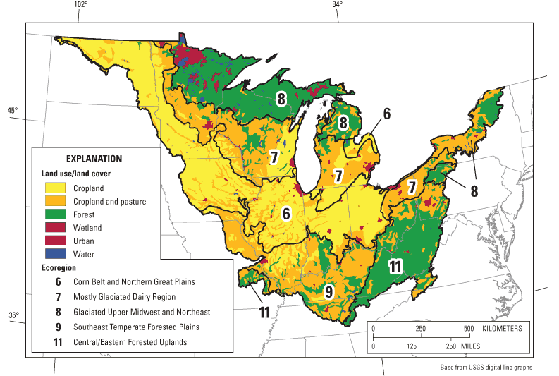
Figure 1. National nutrient ecoregions (U.S. Environmental Protection Agency, 1998) and major land uses in the upper Midwest (U.S. Geological Survey, 2000 and 2004).

Figure 2. Two regionalization schemes considered for wadeable streams in Wisconsin: A, level III ecoregions (Omernik and others, 2000) with major land-use/land-cover categories (Lillesand and others, 1998) and B, environmental phosphorus zones (Robertson and others, 2006).
The nutrient ecoregions proposed by the U.S. Environmental Protection Agency (1998) may define spatial patterns in water quality; however, this regionalization scheme has some inherent problems. Although the boundaries between ecoregions are supposed to represent the differences in a suite of related environmental characteristics (Omernik, 1995), specific boundary lines are often based on differences in a single environmental characteristic and that characteristic may not be the primary one affecting a specific water-quality characteristic. Therefore, greater variations in water quality may occur within an ecoregion than among ecoregions. Second, in defining most ecoregions, the relative importance of each environmental characteristic is often unknown and can vary from one area of the country to another in an unknown way. Therefore, the differences in water quality among ecoregions can be difficult to attribute to any specific environmental characteristic. Finally, for many applications, such as establishing reference conditions for nutrient criteria, the environmental characteristics used to delineate regions of similar water quality should be restricted, as much as possible, to characteristics that are intrinsic, or natural, and are not the result of human activities (U.S. Environmental Protection Agency, 2000a). Here, "reference" water quality refers to background concentrations or the potential water quality that could be achieved in the absence of human activities. By comparing the lines delineating the ecoregions with the land-use patterns in figure 1, it is apparent, however, that land use was the most important characteristic in defining the ecoregions in the upper Midwest. Although the ecoregion delineation is supposed to represent differences in a full suite of environmental characteristics, nutrient ecoregions primarily subdivide the upper Midwest (and Wisconsin) into areas of forest, cropland and pasture, and cropland.
To overcome the problems just described with the USEPA's nutrient ecoregions, SPARTA (SPAtial Regression-Tree Analysis) was developed to define characteristic-specific zones with similar reference water quality for the upper Midwest (Robertson and Saad, 2003) and refined to remove both the direct and indirect effects of land use (Robertson and others, 2006). There are two steps in the SPARTA process to delineate water-quality zones. The first step is to use regression-tree analysis (Breiman and others, 1984) to describe the relations between a single dependent variable (for example, phosphorus (P) concentrations) and various independent variables (for example, clay content of the soil and basin slope) thought to affect the distribution of the dependent variable. The second step of SPARTA is to use the regression-tree results (specific characteristics and breakpoints) to divide the entire study area into zones representing each of the final branches of the analysis.
To refine the SPARTA approach, land-use-adjusted (residualized) water-quality and environmental characteristics were computed and used to remove the direct and indirect effects of land use from the data for each site. Although SPARTA can be applied with only intrinsic or natural characteristics to remove the direct effects of land use as done by Robertson and Saad (2003), these natural characteristics themselves may be strongly correlated with land use. Thus, even if natural characteristics are the only factors included in the analysis, land use can be indirectly incorporated into the results. SPARTA was applied to the land-use-adjusted nutrient data and land-use-adjusted environmental-characteristic data for sites throughout the upper Midwest to develop environmental water-quality zones (Robertson and others, 2006). Because the biota in streams were assumed to be more influenced by P than by total nitrogen (N) concentrations, environmental P zones (EPZs) were examined as an alternative regionalization scheme for the wadeable streams of Wisconsin (fig. 3). The upper Midwest is divided into five EPZs based primarily on the clay content of the soil and secondarily on the slope of the terrain. Wisconsin consists of four major EPZs and one minor EPZ (fig. 2B). Streams in EPZ 1 have basins with the lowest clay content, streams in EPZ 2 have soils with moderate clay content and low-gradient terrain, streams in EPZ 3 have basins with high clay content and low-gradient terrain, and streams in EPZ 4 have basins with moderate clay content and steep terrain. Only a small part of EPZ 5 (basins with high clay content, steep terrain, and high soil erodibility) is in Wisconsin and, therefore, is not examined in detail in this study. Each of these zones contain streams with relatively similar reference P concentrations and with P concentrations that should respond similarly to changes in land use.
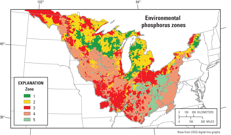
Figure 3. Environmental phosphorus zones (EPZs) in the upper Midwest from Robertson and others (2006).
After relatively homogenous geographic areas are chosen, several approaches have been used to define quantitative nutrient criteria. The approach suggested by the USEPA to define possible criteria is based on the reference or potential water quality of each area. In other words, the criteria should be based on the conditions that are attainable in the geographic location of each stream (U.S. Environmental Protection Agency, 2000a). Reference concentrations for P, N, suspended chlorophyll a (SCHL, also referred to as sestonic chlorophyll), and turbidity have been defined from the frequency distribution of all available data (from USEPA's Storage and Retrieval, STORET, database) for each area. It has been suggested that the lower 25th percentile of all concentration data for an area may represent this reference condition (U.S. Environmental Protection Agency, 2000b). In other words, 25 percent of all the sites have water quality at least as good as this reference condition. It has also been suggested that the upper (highest or worst) 75th percentile of the concentration data for a subset of streams thought to be minimally impacted for a defined area may represent this reference condition. In other words, 75 percent of the minimally impacted sites have water quality at least as good as this reference condition. The final criterion should be between these two concentrations. Another approach to estimate reference concentrations for each relatively homogeneous area is to develop a multiple linear-regression model that relates water quality to various anthropogenic factors or characteristics such as the percentages of agriculture and urban area in the watershed (Dodds and Oakes, 2004). With this approach, the estimated concentration of a constituent occurring in the absence of human activities (in other words, with 0-percent agricultural and 0-percent urban areas) represents the reference concentration. These relations or equations can also be used to place confidence intervals on the reference concentrations.
An alternative approach to defining the nutrient criteria is based on thresholds in the response between nutrient concentrations and biotic indices such as algal productivity (chlorophyll a concentration), water clarity, or diatom or fish biotic indices (U.S. Environmental Protection Agency, 2000a). The biotic community that is present in a stream, however, reflects more than just the nutrient concentrations that are or were present in the stream. The biotic community represents the overall ecological integrity of the stream (in other words, physical, chemical, and biological integrity), and thus provides a broad measure of the aggregate effect of all stressors (Barbour and others, 1999). Biotic communities are controlled by many physical, chemical, and biological factors, though they may be directly affected by only a subset of variables. Watershed characteristics (such as geomorphology, geochemistry, and land use/land cover) control the physical/chemical habitat of the stream where the biota live (Frissell and others, 1986; Poff, 1997). Nutrients have been shown to directly affect the productivity and species composition of primary producers, such as macrophytes and benthic and suspended algae, and indirectly affect the primary and secondary consumers in controlled nutrient-enrichment experiments (for example, Mundie and others, 1991; Peterson and others, 1993; Perrin and Richardson, 1997); however, only limited studies have shown observational linkages between nutrients and the health of the biotic communities in natural streams. Among the limited studies in natural environments, Miltner and Rankin (1998) reported that macroinvertebrate- and fish-community indices were negatively correlated with N and P concentrations in wadeable streams in Ohio. Zorn (2003) reported that P was one of the important variables for predicting the presence or absence of specific fish species in Michigan streams. Heiskary and Markus (2003) also reported significant negative correlations between macroinvertebrate- and fish-community characteristics and P and N concentrations in nonwadeable rivers in Minnesota.
If relations between nutrient concentrations and biotic integrity are used to define criteria, the final nutrient criteria should be chosen to minimize degradation in the biotic integrity of the streams. In other words, the criteria should be the concentrations that would not result in high algal concentrations or degradation of other biotic indices. One of the difficulties in defining nutrient criteria is determining the chlorophyll a concentration or other biotic index values for which a stream is considered degraded or impaired. The assumption made with this biotic-response approach is that each of the subregions in a regional framework also delineates an area with streams whose biotic indices respond in a similar manner to changes in nutrients. Whichever approach is used, the final criteria must be stringent enough to protect the specific site and cause no adverse effects in downstream waters.
Reference nutrient concentrations, the responses in nutrient concentrations to changes in land use, and the biotic responses to changes in nutrients may differ in streams throughout Wisconsin. There would be more confidence in the potential environmental benefits of enforcing nutrient criteria and standards for the State, if the criteria and standards were based on the most appropriate regionalization scheme (such as nutrient ecoregions or EPZs), and if the criteria and standards were based on the appropriate regionally defined thresholds to biotic response. Defined nutrient criteria and thresholds for responsive biotic indices would enable the use of monitoring data to identify streams affected by excessive nutrients and to direct rehabilitation efforts.
The two regionalization schemes being considered for the establishment of nutrient criteria for Wisconsin, level III ecoregions and EPZs, are shown in figure 2. The USEPA developed the preliminary criteria based on median concentrations of all the data measured at each site rather than mean concentrations, because a median value represents the concentration most frequently occurring in the stream, and a statistical summary based on median values reduces the effects of outliers and values reported as less than their respective detection limits. The USEPA has provided preliminary criteria for P, N, SCHL, and turbidity for the national nutrient ecoregions and most level III ecoregions (table 1). The proposed criteria by the USEPA for P, based on the 25th-percentile approach, are 0.033 mg/L for national nutrient ecoregion 7 and 0.010 mg/L for national nutrient ecoregion 8 (same as the NLF ecoregion). The USEPA has refined the P criteria for level III ecoregions in national nutrient ecoregion 7: 0.029 mg/L for NCHF, 0.070 mg/L for DFA, and 0.080 for SWTP (U.S. Environmental Protection Agency, 2000b and 2001).
Table 1. Reference concentrations for total phosphorus, total nitrogen, and suspended chlorophyll a, and turbidity in selected national nutrient and level III ecoregions (U.S. Environmental Protection Agency, 2000b and 2001) and environmental phosphorus zones (EPZs) from Robertson and others (2006).
[USEPA, U.S. Environmental Protection Agency; NCHF, North Central Hardwood Forests; DFA, Driftless Area; SWTP, Southeastern Wisconsin Till Plains; --, no data; NTU, nephelometric turbidity units; FTU, formazin turbidity units; mg/L, milligram per liter; µg/L, microgram per liter]
| Region | USEPA criteria | Reference concentration based on Robertson and others (2006) | |||
|---|---|---|---|---|---|
| Median | Standard error | Upper 95-percent confidence limit | 25th percentile of all sites | ||
|
|
|||||
| Ecoregion 7 | 0.033 | 0.016 | 0.003 | 0.024 | 0.040 |
| NCHF-51a | .029 | -- | -- | -- | -- |
| DFA-52a | .070 | -- | -- | -- | -- |
| SWTP-53a | .080 | -- | -- | -- | -- |
| Ecoregion 8 | .010 | .015 | .002 | .019 | .010 |
| EPZ 1 | -- | .012 | .002 | .017 | .020 |
| EPZ 2 | -- | .021 | .003 | .026 | .030 |
| EPZ 3 | -- | .021 | .004 | .030 | .060 |
| EPZ 4 | -- | .023 | .003 | .030 | .050 |
|
|
|||||
| Ecoregion 7 | 0.54/0.54 | -- | -- | -- | -- |
| NCHF-51a | .46/.71 | -- | -- | -- | -- |
| DFA-52a | 1.88/1.51 | -- | -- | -- | -- |
| SWTP-53a | 1.59/1.30 | -- | -- | -- | -- |
| Ecoregion 8 | .20/.38 | -- | -- | -- | -- |
|
|
|||||
| Ecoregion 7 | 1.7/2.32 | -- | -- | -- | -- |
| NCHF-51a | .84/2.14 | -- | -- | -- | -- |
| DFA-52a | 3.38/2.4 | -- | -- | -- | -- |
| SWTP-53a | --/2.74 | -- | -- | -- | -- |
| Ecoregion 8 | .81/1.3 | -- | -- | -- | -- |
|
|
|||||
| Ecoregion 7 | 1.54/3.50/5.8 | -- | -- | -- | -- |
| NCHF-51a | 1.03/8.76/-- | -- | -- | -- | -- |
| DFA-52a | 1.00/2.32/-- | -- | -- | -- | -- |
| SWTP-53a | .55/3.52/-- | -- | -- | -- | -- |
| Ecoregion 8 | .60/2.60/4.3 | -- | -- | -- | -- |
a USEPA level III ecoregion identification numbers
Robertson and others (2006) estimated median reference P concentrations for the two major national ecoregions and four major EPZs in Wisconsin (fig. 2) by use of the multiple linear-regression approach (previously described). They found that median reference P concentrations for the two national nutrient ecoregions were similar, approximately 0.015–0.016 mg/L. They also found that the four major EPZs could be combined into two zones based on estimated reference P concentrations of 0.012 mg/L for EPZ 1 and approximately 0.021–0.023 mg/L for EPZ 2, EPZ 3, and EPZ 4, and the four major EPZs could be combined into three zones based on the response of P concentrations to changes in land use: EPZ 1 was least responsive, EPZ 2 and EPZ 4 were moderately responsive, and EPZ 3 was most responsive. Streams in EPZ 3, with the highest clay content, had high reference P concentrations (similar to EPZs 2 and 4), but were the most responsive to changes in land use.
In 2001, the U.S. Geological Survey (USGS) and the Wisconsin Department of Natural Resources (WDNR), began a collaborative study to: 1) describe how the nutrient concentrations and biotic-community structure in streams differ throughout Wisconsin; 2) determine which environmental characteristics of watersheds are most strongly related to the distribution of nutrient concentrations in streams; 3) determine reference water-quality and biotic conditions for different areas of the State; 4) determine how the biotic community of streams in different areas of the State respond to changes in nutrient concentrations; 5) evaluate existing regionalization schemes in terms of describing patterns in reference water-quality conditions and patterns in biotic response to changes in nutrient concentrations; and 6) develop new multiparameter biotic indices to predict nutrient concentrations in streams. The ultimate goal of this study is to provide the information needed to guide the development of regionally based nutrient criteria for streams in Wisconsin.
Because the biotic response in streams was expected to vary as a function of stream size, and wadeable streams are sampled with different techniques than nonwadeable streams, the study was divided into two parts. The first part involved sampling 240 wadeable streams in 2001–03, and the second part involved sampling approximately 40 nonwadeable streams in 2003. In this report, the results of the first part of this study are presented: nutrient concentrations and their relations to the biotic integrity of wadeable streams in Wisconsin. The second part of the study will be presented in a separate report.
Because simultaneously collected hydrological, water-quality, and biological data were not available to determine how the biotic integrity of Wisconsin streams is related to changes in nutrient concentrations, a network of streams was selected to represent the wadeable and nonwadeable streams in the level III ecoregions and EPZs in the State. Although some level III ecoregions were combined into larger-scale national nutrient ecoregions and some of the EPZs were combined because there were no statistical differences in reference concentrations or in the responses to changes in land use among some zones in the upper Midwest study (Robertson and others, 2006), each of the level III ecoregions and EPZs were examined separately in this study. The locations of the 240 wadeable streams are shown in figure 4 and listed in appendix 1. To try to obtain streams that represent the range in environmental conditions in Wisconsin, approximately the same number of sites was chosen in each of the level III ecoregions. To try to obtain streams with a wide range in nutrient concentrations, sites in each ecoregion were chosen to try to represent a full range in the percentage of agricultural land, although this was not always possible. Discharge and water quality of each stream were sampled monthly over a 6-month period (May through October). Benthic (attached) algae and diatoms were sampled once during the period. During 2001, 157 streams with the smallest watersheds were sampled (2.2 to 222 km2, but generally less than 90 km2). During 2002, 78 larger streams were sampled (40 to 1,947 km2). In 2003, 42 nonwadeable streams (not discussed in this report) and five additional wadeable streams were sampled (11 to 106 km2). Data on macroinvertebrate and fish populations were not collected as part of this study, but were available from past surveys. A prerequisite for site selection was that the macroinvertebrate and fish populations in the stream had been sampled during the past 5 years.
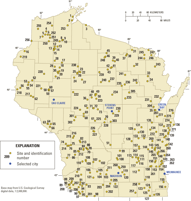
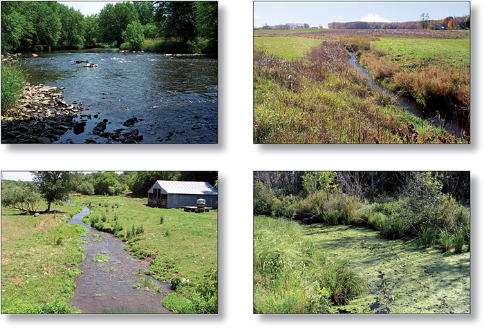
Figure 4. Sites on wadeable streams in Wisconsin included in this study. Water-quality and biotic data for each site are given by site identification number in the appendixes.
For each site, the drainage basin was digitized and a geographic information system (GIS) was used to describe the environmental characteristics of the watershed. Various multivariate statistical approaches were then used to determine how the environmental characteristics of the watershed were related to water quality and biotic-community structure. The data were used to determine which stratification scheme (level III ecoregions or EPZs) best describes the distributions in reference nutrient concentrations and the responses in nutrient concentrations to changes in land use. Reference concentrations of P, N, and SCHL, and water clarity were estimated by use of the multiple linear-regression approach and the 25th-percentile approach for the best regionalization scheme. Reference values for the biotic indices were estimated by use of the 75th-percentile approach by examining the values of the biotic indices at minimally impacted sites (sites with nutrient concentrations at or below the estimated reference concentrations). Water-quality data were statistically compared with biotic indices describing the suspended and benthic algae, diatoms, macroinvertebrates, and fish to determine how the biotic integrity of streams is related to changes in nutrient concentrations, and whether or not thresholds in P and (or) N concentrations can be defined above which the biology is adversely affected. Two new multiparameter indices were then developed to estimate P and N concentrations in streams on the basis of the biotic-community structure.
Streamflow and water quality in each stream were sampled monthly over a 6-month period (May through October). Each site was sampled near the middle of the month regardless of flow conditions. During each visit, discharge and field parameters (specific conductance, water temperature, dissolved oxygen, and pH) were either measured or estimated and a water-quality sample was collected.
Discharge was determined at each site with a current meter (Rantz and others, 1982), with a stage/discharge relation for a continuous-recording gaging station at the site, or estimated from a nearby site. If the site was not wadeable because of high flow and did not have a continuous-recording gage, the discharge was estimated from a nearby streamflow-gaging station by use of relations between previous discharge measurements at the site and at the nearby station.
Specific conductance, water temperature, dissolved oxygen, pH, and, at some sites, turbidity were measured in the field at the time of sampling by use of a multiparameter meter. The meters were calibrated each day before use. Water clarity was measured by use of a 120-cm Secchi tube (also referred to as a transparency tube, U.S. Environmental Protection Agency, 2004). The Secchi tube was held into the flowing stream and filled. The tube was then held perpendicular to the ground and drained until the Secchi disk at the bottom of the tube became visible. The water level in the tube was read to the nearest centimeter and defined as the Secchi tube depth (SD). If the disk was visible when the tube was full, the value was reported as greater than 120 cm.
All water samples were collected by use of the equal-width-increment (EWI) method with a hand-held DH-59 depth-integrating sampler (Edwards and Glysson, 1999), except when stream conditions were not appropriate (stream velocity less than approximately 0.45 m/s, maximum depth less than 0.15 m, or the stream was nonwadeable); in this case, a grab sample was collected with an open bottle at the center of the flow. Samples were then split into appropriate bottles for lab analysis. Samples to be analyzed for dissolved constituents were filtered in the field through 0.45-µm membrane filters. Samples to be analyzed for SCHL were obtained by filtering a known volume of water through a 5-µm membrane filter. The filter was then placed in a labeled petri dish and wrapped in aluminum foil. All samples were chilled until they were delivered to the Wisconsin State Laboratory of Hygiene for analysis, except samples to be analyzed for SCHL, which were frozen, kept in the dark, and delivered to the WDNR Research Laboratory. All samples were analyzed for P, dissolved phosphorus (DP), total Kjeldahl nitrogen (TKN), dissolved nitrite plus nitrate nitrogen (NO3-N), dissolved ammonia nitrogen (NH4-N), and SCHL. In July of 2002, samples were also collected for analysis of suspended sediment. All chemical analyses of water samples (except SCHL) were done by the Wisconsin State Laboratory of Hygiene in accordance with standard analytical procedures described in the "Manual of Analytical Methods, Inorganic Chemistry Unit" (Wisconsin State Laboratory of Hygiene, 1993). At the WDNR Research Laboratory, the filters for SCHL analysis were placed in tubes containing 90 percent acetone, stored at least 24 hours, sonicated for 15 minutes, and stored an additional 24 hours in a freezer. The trichromatic chlorophyll a content of the samples was determined by means of a USEPA-approved method (Greenberg and others, 1992). Throughout this report, the water-chemistry, water-clarity, and SCHL data are collectively referred to as "water-quality data." All water-quality data were input into the USGS National Water Information System (NWIS) (U.S. Geological Survey, 1998).
Samples for benthic chlorophyll a (BCHL) and periphytic-diatom analyses were collected once during August or September. Care was taken to avoid collecting samples within 2 weeks of appreciable rainfall to minimize the potential effect of scouring. Samples were collected by brushing a known area of three to five rocks with a toothbrush. Following collection, the samples were placed on ice and kept in the dark. Within 12 hours of sampling, the sample was diluted to a known volume with distilled water, homogenized in a blender, and a portion was filtered through two 3–5 µm glass-fiber filters. One filter was placed in 90 percent acetone and was analyzed for its acid-corrected chlorophyll a content (BCHL) by means of a USEPA-approved monochromatic method (Greenburg and others, 1992). The other filter was used for the determination of ash-free dry weight. This sample was dried overnight at 105°C and ashed at 550°C for 1 hour. The sample was weighed before and after ashing. Because of either lack of suitable substrate or lack of water at the time of collection, BCHL samples were collected from only 199 sites.
The sample for microscopic analysis of the diatom assemblage was obtained from a portion of the homogenized sample used for BCHL analysis; however, if rocks were not available, samples were collected from sticks. The sample was preserved with Lugols solution and cleaned with hydrogen peroxide and potassium dichromate (van der Werff, 1955). A portion of the diatom suspension was dried on a cover slip and mounted in Naphrax. Specimen were identified and counted under an oil-immersion objective (1,400 or 1,750X). At least 300 diatoms were counted from two slides in each sample. The keys used to identify the species included Patrick and Reimer (1966, 1975), Camburn and others (1984–86), Dodd (1987), and Krammer and Lange-Bertalot (1986, 1988, 1991a,b). Because of either lack of coarse substrate or lack of water at the time of collection, samples were collected from only 214 sites.
Physical-habitat and fish data were collected by the WDNR once at each site between 1997 and 2002. The physical habitat was determined for a stream length equal to 35 times the mean stream width, or a minimum of 100 m. This length is generally sufficient to encompass about three meander sequences (Simonson and others, 1994; Wang and others, 1996). The physical habitat and fish were quantified between late May and late August when low flows facilitated effective sampling and large-scale seasonal fish movement was unlikely to occur (Lyons and Kanehl, 1993). At each site, 30 physical-habitat characteristics, including channel morphology, bottom substrates, cover, bank conditions, riparian vegetation, and land cover were measured or visually estimated along 12 transects by use of standard procedures (Simonson and others, 1994). The entire length of each site was electrofished with either two backpack units in tandem or a single tow-barge unit with three anodes (Lyons and Kanehl, 1993; Simonson and Lyons, 1995). Efforts were made to collect all of the fish greater than or equal to 25 cm in length. All captured fish were identified to species, counted, and weighed in aggregate by species.
Macroinvertebrate samples were collected by the WDNR once at each site between 1999 and 2002. Two types of macroinvertebrate samples were collected according to procedures described by Hilsenhoff (1988). Samples were generally collected from each site during low flow in early October by use of a 600-µm mesh D-frame kick net. The first sample was collected from riffles or rocky substrates. If rocky substrates were not present, then vegetative snags (areas with overhanging grasses, logs, woody debris, and leaf packs) were sampled to ensure that the sample was from the most representative habitat at each site. The second sample was collected only from snags to ensure that these data were comparable between all sites because rocky substrates were not always present.
Samples from riffle or rocky substrates were collected by placing the net on the stream bottom and kicking an area immediately upstream of the net to dislodge the macroinvertebrates and wash them into the net. In addition, individual rocks were picked up and the attached macroinvertebrates were removed and added to the sample. This process was repeated in at least three locations within the same riffle or different riffles until at least 200–300 organisms were collected. Samples were collected in snags by placing a net in the water column downstream of the snag, where it would collect most of the dislodged debris. The snags were then disturbed by scraping or shaking them with a net, hands, or feet. At each site, all available snag types at multiple locations were sampled, with first consideration given to larger snags in higher water-velocity habitats.
Samples were sorted and identified at the laboratory of Dr. Stanley Szczytko at the University of Wisconsin, Stevens Point. The samples were placed in a glass pan positioned over a 6.5-cm2 grid. All of the organisms from randomly chosen grid squares were selected until a minimum of 125 organisms having tolerance values cited in the literature (such as the values in Hilsenhoff, 1988) were picked, or, until the entire sample was sorted. All of the picked organisms were counted and identified to the species or the lowest taxonomic level possible.
Watershed boundaries for the sampled streams were manually digitized from 1:24,000-scale USGS topographic quadrangle maps. The environmental characteristics thought to affect the water quality and biology in the streams were compiled for each watershed used in this study: land use/land cover (Lillesand and others, 1998); soil characteristics (from the USSOILS digital coverage of the State Soil Geographic, STATSGO, data base; Schwarz and Alexander, 1995); types of surficial deposits (Fullerton and others, 2003); annual air temperature and precipitation (National Climatic Data Center, 2002); mean land-surface slope (based on 30-m DEM data resampled to 100 m; U.S. Geological Survey, 1999); and average annual runoff (Gebert and others, 1987).
Point-source loadings of phosphorus upstream of each sampling site (PtS) were estimated from monthly mean P concentrations and monthly mean discharge volumes as reported by the dischargers (for example, wastewater-treatment plants and cheese factories) in their Discharge Monitoring Report with the WDNR (James Baumann, Wisconsin Department of Natural Resources, written commun., 2004). The number of concentrations and discharge volumes reported in a month varied with the size and type of discharger and ranged from one sample per month to daily samples. For sites where P concentrations were not required to be measured and, therefore not reported, the P concentrations were estimated based on the size and type of discharger.
All basin characteristics were compiled in digital form by use of a GIS. A digital coverage of each watershed was used to compute the average or percentage value for each environmental characteristic, including the PtS for each of the 240 watersheds. A summary of the environmental characteristics (with the specific metric describing each environmental characteristic) for all of the watersheds used in this study is given in table 2.
Table 2. Summary statistics for median monthly water-quality and environmental (anthropogenic/land-use, basin, soil, and surficial-deposit) characteristics of the watersheds of the sites in the studied wadeable streams in Wisconsin.
[mg/L, milligram per liter; log, logarithm to base 10 transformation; µg/L, microgram per liter; C, Celsius; µS/cm, microSiemen per centimeter; cm, centimeter; (m3/s)/km2, cubic meter per second per square kilometer; km2, square kilometer; mm, millimeter; mm/year, millimeter per year; --, unitless; %, percent; mm/hr, millimeter per hour; kg/km2, kilogram per square kilometer; >, greater than; no PtS, only sites with less than 12 kg/km2 of point-source loading of phosphorus are included in this part of the analysis; summary statistics based on monthly values]
| Characteristic | Unit | Transformation | Count | Median | Mean | Standard deviation | Minimum | Maximum |
|---|---|---|---|---|---|---|---|---|
|
|
||||||||
| Total phosphorus | mg/L | log | 240 | 0.085 | 0.116 | 0.144 | 0.012 | 1.641 |
| Total phosphorus (no PtS) | mg/L | log | 234 | .082 | .105 | .097 | .012 | .741 |
| Dissolved phosphorus | mg/L | log | 240 | .050 | .079 | .122 | .004 | 1.495 |
| Dissolved phosphorus (no PtS) | mg/L | log | 234 | .050 | .069 | .074 | .004 | .553 |
| Total nitrogen | mg/L | log | 240 | 1.695 | 2.807 | 2.860 | .131 | 21.260 |
| Dissolved nitrite plus nitrate | mg/L | log | 240 | 1.048 | 2.086 | 2.865 | .005 | 20.550 |
| Dissolved ammonia | mg/L | log | 240 | .029 | .039 | .044 | .007 | .040 |
| Total Kjeldahl nitrogen | mg/L | log | 240 | .563 | .675 | .414 | .070 | 2.350 |
| Suspended chlorophyll a | µg/L | log | 240 | 2.27 | 3.23 | 4.06 | .40 | 38.01 |
| Water temperature | C | none | 240 | 15.7 | 15.5 | 2.0 | 9.3 | 21.6 |
| Specific conductance | µS/cm | none | 240 | 478 | 455 | 284 | 27 | 1,405 |
| Secchi tube deptha | cm | none | 240 | 112.0 | 97.3a | 28.9 | 23.5 | >120 |
| Flow per unit area | (m3/s)/km2 | log | 240 | .007 | .009 | .011 | .001 | .122 |
|
|
||||||||
| Urban | % | none | 240 | .00 | .01 | .01 | .00 | .14 |
| Agriculture (row crops) | % | none | 240 | .20 | .24 | .21 | .00 | .78 |
| Agriculture (other) | % | none | 240 | .20 | .19 | .15 | .00 | .57 |
| Total agriculture | % | none | 240 | .46 | .42 | .31 | .00 | .94 |
| Grassland | % | none | 240 | .09 | .10 | .08 | .00 | .39 |
| Wetland (open) | % | none | 240 | .02 | .04 | .06 | .00 | .48 |
| Wetland (forested) | % | none | 240 | .03 | .07 | .10 | .00 | .85 |
| Barren | % | none | 240 | .01 | .02 | .02 | .00 | .21 |
| Forest (all) | % | none | 240 | .31 | .40 | .31 | .01 | .99 |
| Point-source loading of phosphorus | kg/km2 | log | 240 | .00 | 1.47 | 6.44 | .00 | 73.62 |
|
|
||||||||
| Watershed area | km2 | log | 240 | 26.4 | 121.9 | 261.8 | 2.2 | 1947.1 |
| Air temperature | C | none | 240 | 6.9 | 6.5 | 1.4 | 3.7 | 9.2 |
| Precipitation | mm | none | 240 | 837 | 836 | 37 | 743 | 926 |
| Runoff | mm/yr | none | 240 | 229 | 246 | 50 | 152 | 366 |
| Basin slope | degrees | none | 240 | 5.92 | 6.85 | 3.49 | 1.35 | 16.04 |
| |
||||||||
| Clay content | % | none | 240 | 18.10 | 19.07 | 10.58 | 3.43 | 41.80 |
| Erodibility | -- | none | 240 | .28 | .26 | .07 | .11 | .40 |
| Organic-matter content | % | none | 240 | 3.83 | 5.19 | 5.06 | .30 | 31.02 |
| Permeability | mm/hr | none | 240 | 58.32 | 84.57 | 66.41 | 16.00 | 307.71 |
| Soil slope | % | none | 240 | 6.03 | 7.49 | 4.59 | 1.02 | 23.03 |
| |
||||||||
| Nonglacial deposits | % | none | 240 | .00 | .23 | .41 | .00 | 1.00 |
| Clay | % | none | 240 | .00 | .12 | .30 | .00 | 1.00 |
| Loam | % | none | 240 | .00 | .08 | .26 | .00 | 1.00 |
| Peat | % | none | 240 | .00 | .01 | .04 | .00 | .42 |
| Sand | % | none | 240 | .26 | .37 | .40 | .00 | 1.00 |
| Sand and gravel | % | none | 240 | .01 | .19 | .28 | .00 | 1.00 |
a All values greater than 120 cm were set to 120 cm for computation of summary statistics, which result in the mean values being biased low.
All of the water-quality data collected in this study were input into the USGS NWIS database (U.S. Geological Survey, 1998) and are summarized in appendix 1. In computing summary statistics, all of the data were used regardless of whether or not flow could be detected. During some samplings, the water in the streams was found to have dried up, and no water-quality data were collected. All data reported as less than the detection limit were set to one-half of the detection limit, and all SD data greater than 120 cm were set to 120 cm prior to any statistical and graphical analyses.
Physical-habitat data were summarized into: mean wetted width, depth, thalweg depth, and stream gradient; the percentage of the stream reach with riffles, runs, or pools; the mean depth of sediment; the percentage of the bottom of the stream reach composed of different substrates, embedded rocky substrate, and covered by algae or macrophytes; the percentage of the stream reach that contains fish cover, is shaded, and that has streambank erosion; and buffer width (Simonson and others, 1994). The physical-habitat data for each site are summarized in appendix 2.
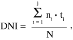
Three metrics were used to summarize the diatom-community data: the Diatom Nutrient Index (DNI), the Diatom Siltation Index (DSI; Bahls, 1992), and the Diatom Biotic Index (DBI). The DNI computations are based on tolerance values assigned to individual taxa. DNI values range from 1 to 6, with 1 representing species typically found with the lowest nutrient concentrations (oligotrophic, good water quality) and 6 typically representing species found with the highest nutrient concentrations (hypereutrophic, poor water quality). The values for Wisconsin diatoms (appendix 3) were generated largely from Van Dam and others (1994), but values were also assigned based upon experience with the diatom communities in Wisconsin. If no autecological data were known, the taxa were not assigned a value and were not included in the DNI calculation. Because the index is based upon relative abundance, rare species have little effect on the final index value. The formula used to calculate DNI value is
 |
(1), |
where
ni = number of individuals of species i;ti = tolerance-index value for species i;
j = total number of species in the sample with tolerance-index values; and
N = total number of individuals in the sample having tolerance-index values.
The second metric for the diatom community is the Diatom Siltation Index (DSI). This index is based on the sum of all individuals in the Navicula (including Cavinula, Chamaepinnularia, Craticula, Diadesmis, Fallacia , Fistulifera, Geissleria, Hippodonta, Kobayasiella, Luticola, Mayamaia, Placoneis , and Sellaphora ), Nitzschia (including Psammodictyon and Tryblionella ), and Surirella taxa. These taxa were chosen because they have good motility; therefore, this metric reflects the degree of siltation in a reach (Bahls, 1992). The scale for the index is 0–100 with lower values indicating less silt and thus better water quality.
To assess stream biotic integrity, a multimetric index called the Diatom Biotic Index (DBI) was created. The DBI is based on both diatom indices, DNI and DSI. For computing the DBI, each metric was standardized to the 95th percentile for a number of reference sites and then the two metrics were averaged. For sites with an individual metric exceeding its 95th percentile, the metric was set to 100. The scale of the DBI is 0 to 100, with higher values indicating better biotic integrity. The DBI is intrinsically designed to be sensitive to nutrient enrichment and the effects of sedimentation. The reference sites used to standardize the metric were chosen by combining the northern ecoregions (NLF, NCHF) and the southern ecoregions (DFA, SWTP). Reference sites for the southern ecoregions were those where P concentrations for August were less than or equal to 0.050 mg/L. For the southern ecoregions, there were 13 reference sites and 105 sites with P concentrations exceeding 0.050 mg/L. Reference sites for the northern ecoregions were sites with less than or equal to 10-percent agriculture in the watershed. For the northern ecoregions, there were 42 reference sites and 55 sites with more than 10-percent agriculture.
Six common measures were used to summarize the macroinvertebrate data: the Hilsenhoff Biotic Index (HBI; Hilsenhoff, 1988) and five other macroinvertebrate indices based on the percentage or total number of individuals of various groups or species that were counted in the samples (for example, Ohio Environmental Protection Agency, 1988; Kerans and Karr, 1994; Barbour and others, 1999; and Weigel, 2003). The HBI is an abundance-weighted tolerance index based on the tolerance of each macroinvertebrate taxon to organic pollution and dissolved oxygen depletion. HBI values range from 0 to 10, with higher values indicating more degraded water quality. The five other macroinvertebrate indices included the percentage of individuals that were either Ephemeroptera, Plecoptera, or Trichoptera (EPTN%), the percentage of taxa that were Ephemeroptera, Plecoptera, or Trichoptera (EPTTX%), the percentage of individuals that were scrapers (SCRAP%), the percentage of individuals that were shredders (SHRED%), and the total number of taxa (TAXAN). For each site, each of these indices was computed for the riffle and snag samples separately, and then an average value was computed. The macroinvertebrate indices for each site are summarized in appendix 4.
Eight community measures were computed to summarize the fish data. Two measures described the quantity of fish caught: total number of fish caught (FISHN) and total number of species caught (FISHSPEC). Five indices described feeding and tolerant classifications: the percentages of top carnivores (CARN%), insectivores (INSECT%), and omnivores (OMNI%), and the percentages of pollution-tolerant (TOL%) and pollution-intolerant (INTOL%) fish (based on Lyons, 1992; and Lyons and others, 1996). In addition, the fish Index of Biotic Integrity (IBI) score was computed by use of both the cold-water (Lyons and others, 1996) and warm-water (Lyons, 1992) versions. Because all of the sites were not classified as a warm-water, cool-water, or cold-water fishery and a cool-water version of the IBI is not available for Wisconsin, the higher of the two IBI scores was used as the site's fish IBI value. The use of different versions of the IBI compensates for different fish assemblages in different thermal regimes. Differences in the other fish indices represent broad feeding and pollution-tolerance classifications; therefore, the metrics in streams with very different species are comparable. The fish metrics for each site are summarized in appendix 4.
The SAS statistical software package (SAS Institute, Inc., 1989) was used for all statistical analyses except for the redundancy analyses, which were done with the CANOCO statistical software package (ter Braak and Smilauer, 2002), and the regression-tree analyses, which were done with the SPLUS statistical software package (Lam, 2001).
Before statistical analyses, all water-quality data except the SD data were logarithmically transformed (base 10) to improve the normality of the data. This transformation improved the normality of the data although not always to the 5-percent-significance level (Shapiro-Wilk normality test). In addition, all chlorophyll a data, point-source data, and watershed areas were logarithmically transformed prior to statistical analyses.
Spearman correlation analyses were used to determine the relation between each water-quality characteristic and biotic index and each environmental characteristic. This nonparametric procedure was chosen to reduce the influence of the assumption of normal-data distributions. Sequential Bonferroni tests were used to determine the statistical significance of the correlations to eliminate the effects of the number of tests on the significant level (Rice, 1989). Pearson correlation analyses were also used to determine the relation between each water-quality characteristic and each environmental characteristic prior to the use of multiple regressions and forward stepwise-regression analysis (with p < 0.05 as the critical level for entry). This procedure was used to determine the magnitude of the interaction between environmental characteristics and water-quality characteristics, as well as to determine the best multivariate relation to estimate concentrations at a specific site as a function of the environmental characteristics in its watershed.
Many studies (such as Robertson and others, 2006, and this study), have shown that land use not only directly affects water quality, but it is often strongly correlated with the environmental characteristics used to define regions of similar water quality (indirect effects of land use). Therefore, in order to determine the relation between water quality and the nonanthropogenic or natural characteristics, a simultaneous partial-residualization approach, related to partial correlation, was used to remove the agricultural and urban effects from the concentrations of P and N and from the measures of each of the environmental characteristics.
In simple regression, the relation between the dependent variable Y (for example, P) and a predictor variable X1 (for example, the clay content of the soil in the basin) can be measured by the sample correlation rYX1. If the variable X1 is regressed on the variable X2 (for example, the percentage of agricultural area), the estimated regression equation X1,2 = ß0 + ß1X2 would be obtained. To adjust X1 for the effects of X2, a "residualized X1", X1*, can be obtained by computing X1* = X1 – X1,2. In a manner similar to simple correlation, the strength of the relation between Y and X1 adjusted for X2 (in this case, land use) can be obtained by the correlation between the residuals for Y on X2 (Y*) and the residuals for X1 on X2 (X1*). The resulting correlation is the partial correlation of Y and X1 adjusted for X2; the strength of the relation between Y and X1 has been adjusted for the effects of X2. This approach, described by Weisberg (1980), is easily extended to control for more than one variable; X2 can be replaced by an arbitrary set of variables. In this study, the residualization approach was used to remove the effects of the percentages of agriculture and urban areas and PtS (logarithmically transformed point-source loading in the basin) to enable the relations between the dependent variables P, N, SCHL, and SD and all of the nonanthropogenic environmental characteristics to be further examined. This approach was not used to examine relations between environmental characteristics and the biotic indices. Spearman correlations and forward stepwise regressions were done with raw data and with residualized data to determine which environmental characteristics best described the distribution of each water-quality characteristic.
In traditional linear-regression analysis, a continuous dependent variable is assumed to be a linear function of a set of independent variables. This is often an unrealistic assumption, and departures from linearity can result in underestimating, or completely discounting, important independent variables. Although departures from linearity can be addressed to some extent by trial-and-error data transformations, this approach becomes problematic when independent variables interact in multiple dimensions. The method of regression-tree analysis (Breiman and others, 1984) prevents these problems by not incorporating the assumptions about the shapes of the relations between a dependent variable and one or more independent variables. Regression-tree analysis sequentially partitions the values of each independent variable into two groups, computes mean values of the dependent variable for each group, and then computes square errors for each partition. At each step, all of the independent variables are scanned, and the independent variable and its breakpoint that minimize the least-square-error criterion are chosen. In a manner similar to the F-statistic in an analysis of variance, the least-square-error criterion is used to identify breakpoints that maximize the variance of the interpartition means relative to the intrapartition variance. This process partitions the independent-variable space into increasingly homogeneous regions (branches on a tree). The end result of this sequential process is a branching diagram. If only one independent variable is used (for example, the concentration of P or N) at each step in the analysis, the best breakpoint for the independent variable is defined as the value which subdivides values of the dependent variable (for example, IBI) into the two groups with the maximum difference in their mean values. This breakpoint represents the threshold in the response of the dependent variable.
Regression-tree analyses were done with various dependent variables (SCHL, SD, and various biotic indices) and the corresponding independent variables (nutrient concentrations) to determine breakpoints or thresholds in the responses of the dependent variables to changes in specific nutrient concentrations. In the analysis, the minimum number of sites used to define a subgroup was set to 25 to avoid creating small outlier groups. Regression-tree analysis was also used to determine the value (threshold) below which PtS had minimal effect on P concentrations.
Redundancy analysis (RDA) is a form of direct-gradient analysis that describes the variation between two multivariate data sets (for example, water-quality and environmental characteristics; ter Braak and Prentice, 1988). In RDA, the site scores from a principal-component analysis are regressed on a specified set of environmental characteristics, and the fitted values of the regression become new site scores for the following iteration; therefore, the principal component analysis is constrained by the environmental variables (Jongman and others, 1987). RDA was used in this study to quantify the variance in the dependent variables (for example, water-quality characteristics) explained by the independent variables (for example, environmental characteristics) and to determine which environmental characteristics best explained the variance in water quality. In addition, partial RDA (Richards and others, 1996) was used to determine the fraction of the variance in the water-quality characteristics explained by specified categories of the environmental characteristics (such as land-use, basin, and soil/surficial-deposit characteristics), and to determine the fraction of the variance in populations of specified groups of the biotic community (such as benthic chlorophyll a concentrations and populations of diatoms, macroinvertebrates, and fish) explained by specified categories of environmental characteristics (such as nutrient characteristics and environmental characteristics). Monte Carlo permutation tests with 99 iterations, the default number of iterations in CANOCO, were used to determine the validity of the total and partial RDA results. Monte Carlo tests were done by permutating the assignment of the independent (environmental) data to the dependent (water-quality or biological) data randomly and repeating the ordinations (Richards and others, 1996; Johnson and others, 1997).
To determine whether any apparent differences among groupings of data (such as reference sites compared to nonreference sites) were statistically significant, the nonparametric Kruskal-Wallis rank analysis of variance test was used, followed by a Tukey multiple-comparison procedure (SAS Institute, Inc., 1989). For all statistically significant differences, the probability of their occurring by chance was less than 5 percent (p < 0.05), unless otherwise specified.
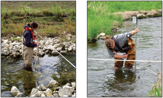
|
Median monthly concentrations of total P ranged from 0.012 to 1.641 mg/L. The overall median and mean were 0.085 and 0.116 mg/L, respectively. Highest concentrations were measured in the central part of the State, especially south of Green Bay (fig. 5). High concentrations were also measured in the southwestern part of the State. The lowest P concentrations were measured in the northern one-third of the State. The highest P concentrations were measured in June and July, and the lowest concentrations were measured in October (table 3).
Median monthly concentrations of DP ranged from 0.004 mg/L (less than the 0.005 mg/L detection limit) to 1.495 mg/L (table 2). The overall median and mean were 0.050 and 0.079 mg/L, respectively. The distribution and seasonality in DP concentrations were similar to total P concentrations (table 3). DP concentrations were strongly correlated to total P concentrations. Pearson correlation coefficients (r values) between DP and P ranged from 0.90 in June to 0.98 in September. DP represented about 53 to 62 percent of the phosphorus during May through July and about 70 percent during August through October.
Table 3. Median and average monthly concentrations for total and dissolved phosphorus, suspended chlorophyll a, total nitrogen, nitrite plus nitrate, ammonia, and Kjeldahl nitrogen, and Secchi tube depths in the studied wadeable streams in Wisconsin.
[mg/L, milligram per liter; µg/L, microgram per liter; cm, centimeter; >, greater than; all concentrations are in mg/L, except chlorophyll a, which is in µg/L, and Secchi tube depth, which is in cm]
| Total phosphorus | Dissolved phosphorus | Chlorophyll a | Secchi tube depth | |||||
|---|---|---|---|---|---|---|---|---|
| Month | Median | Average | Median | Average | Median | Average | Median | Average |
| May | 0.070 | 0.115 | 0.037 | 0.071 | 2.890 | 4.420 | 105.0 | 89.8 |
| June | .107 | .164 | .058 | .101 | 2.120 | 3.120 | 88.5 | 79.6 |
| July | .092 | .143 | .052 | .089 | 3.042 | 7.885 | 90.0 | 82.9 |
| August | .088 | .138 | .059 | .096 | 2.168 | 5.096 | > 120 | 92.9 |
| September | .075 | .120 | .049 | .085 | 1.773 | 3.336 | > 120 | 101.1 |
| October | .049 | .101 | .035 | .070 | 1.546 | 2.922 | > 120 | 107.9 |
| Total nitrogen | Nitrite plus nitrate | Ammonia | Kjeldahl nitrogen | |||||
| Month | Median | Average | Median | Average | Median | Average | Median | Average |
| May | 1.589 | 2.919 | 0.911 | 2.120 | 0.030 | 0.061 | 0.700 | 0.800 |
| June | 2.110 | 3.949 | 1.120 | 2.500 | .033 | .049 | .790 | .949 |
| July | 1.740 | 2.851 | .903 | 2.083 | .032 | .067 | .560 | .768 |
| August | 1.573 | 2.634 | .788 | 1.919 | .031 | .062 | .525 | .715 |
| September | 1.622 | 2.750 | .987 | 2.115 | .031 | .060 | .510 | .650 |
| October | 1.657 | 2.834 | 1.080 | 2.229 | .027 | .046 | .470 | .606 |
Median monthly concentrations of N ranged from 0.131 to 21.260 mg/L (table 2). The overall median and mean were 1.695 and 2.807 mg/L, respectively. The highest median N concentrations were measured in the southern quarter of the State and the eastern half of the State (fig. 5). The lowest N concentrations were found in the northern quarter of the State. The highest N concentrations were measured in June, but no consistent seasonal patterns were measured (table 3).
Median monthly concentrations of NO3-N ranged from 0.005 mg/L (less than the 0.010 mg/L detection limit) to 20.550 mg/L (table 2). The overall median and mean were 1.048 and 2.086 mg/L, respectively. Median monthly concentrations of NH4-N ranged from 0.007 mg/L (less than the 0.013 mg/L detection limit) to 0.040 mg/L. The overall median and mean were 0.029 and 0.039 mg/L, respectively. Median monthly concentrations of TKN ranged from 0.070 mg/L (less the 0.140 mg/L detection limit) to 2.350 mg/L. The overall median and mean were 0.563 and 0.675 mg/L, respectively. Most of the nitrogen was in the form of NO3-N (ranging from 63 percent in June to 73–79 percent in other months). Highest NO3-N and TKN concentrations were measured in June, but no consistent seasonal patterns were measured in any form of nitrogen.
Median monthly concentrations of SCHL ranged from 0.40 to 38.01 µg/L (table 2). The overall median and mean were 2.27 and 3.23 µg/L, respectively. Highest SCHL concentrations were measured in the central and eastern parts of the State, especially south of Green Bay and north of Milwaukee (fig. 5). Lowest SCHL concentrations were measured in the northern one-third of the State and in the southwestern part of the State. Highest SCHL concentrations were measured in July, and lowest concentrations were measured in September and October (table 3).
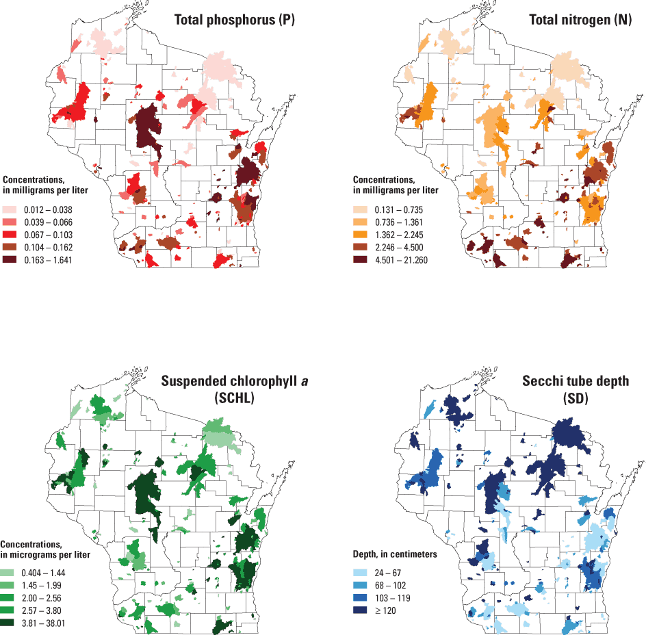
Figure 5. Distributions (quintiles) of median monthly total phosphorus (P), total nitrogen (N), and suspended chlorophyll a concentrations (SCHL), and Secchi tube depth (SD) for the studied wadeable streams in Wisconsin. (Note: the upper 40 percent of SDs were all greater than or equal to 120 centimeters.)
Median monthly SDs ranged from 23.5 cm to greater than 120 cm (table 2). Many sites consistently had clarities greater than the length of the Secchi tube. The overall median and mean were 112 and 97.3 cm, respectively. Highest SDs (the best clarities) were measured in the northern half of the State (fig. 5). Lowest SDs (the worst clarities) were measured in the southwestern and central parts of the State and south of Green Bay. Lowest SDs were measured during May through July, and the highest SDs were measured during August through October (table 3).
Spearman correlation coefficients (rs values) between median water-quality characteristics are shown in table 4. P and DP were significantly correlated with N, NO3-N, NH4-N, and TKN (rs values ranged from 0.36 to 0.61). Correlations between P and the nitrogen species were slightly stronger than between DP and the nitrogen species. Concentrations of N were strongly correlated (rs = 0.91) to NO3-N because NO3-N was the major form of nitrogen. Concentrations of NH4-N and TKN were more strongly correlated to one another (rs = 0.66) and to P (rs ~ 0.6) than they were to total N and NO3-N (rs ~ 0.1–0.3). NH4-N is part of TKN; therefore, a correlation between these two forms of nitrogen was expected. Total organic nitrogen was computed by subtracting the NH4-N concentration from the TKN concentration. Total organic nitrogen and NH4-N were still strongly correlated with one another (rs = 0.62). Concentrations of P and DP were also significantly correlated with the PtS in the basin (rs ~ 0.3). The six streams with PtS values higher than 12 kg/km2 had some of the highest measured P (ranging from 0.17 to 1.64 mg/L) and DP concentrations (ranging from 0.098 to 1.49 mg/L). Annual PtS below 12 kg/km2 had little effect on the concentrations of P and DP in the streams (on the basis of results from regression-tree analyses and graphical examination of the data). Omitting the six streams with PtS greater than 12 kg/km2 from the analyses, however, had little effect on the correlations with the other characteristics (table 4).
Table 4. Spearman correlation coefficients (rs) between median concentrations of total phosphorus, dissolved phosphorus, total nitrogen, nitrite plus nitrate, ammonia, total Kjeldahl nitrogen, median Secchi tube depths, suspended chlorophyll a concentrations, percentages of urban and agricultural areas, point-source loadings of phosphorus, and specific environmental (anthropogenic/land-use, basin, soil and surficial-deposit) characteristics for the studied wadeable streams in Wisconsin.
[P, total phosphorus; DP, dissolved phosphorus; N; total nitrogen; NO3-N, nitrite plus nitrate; NH4-N, ammonia; TKN, total Kjeldahl nitrogen; SD, Secchi tube depth; SCHL, suspended chlorophyll a concentration; % Urb, percentage of urban area; % Ag, percentage of agricultural area; PtS, point-source loading of phosphorus in kilograms per square kilometer; <, less than; no PtS, only sites with less than 12 kilograms per square kilometer of point-source loading of phosphorus are included in analysis; all values with an absolute value greater than 0.22 are statistically significant at p < 0.05; all values with an absolute value greater than 0.4 are in bold]
| Characteristic | P |
P (no PtS) |
DP |
DP (no PtS) |
N | NO3-N | NH4-N | TKN | SD | SCHL | % Urb | % Ag | PtS |
|---|---|---|---|---|---|---|---|---|---|---|---|---|---|
|
|
|||||||||||||
| Total phosphorus | 1.00 | 1.00 | 0.95 | 0.95 | 0.54 | 0.38 | 0.61 | 0.56 | -0.57 | 0.44 | 0.14 | 0.67 | .29 |
| Dissolved phosphorus | 0.95 | 0.95 | 1.00 | 1.00 | .51 | .36 | .55 | .52 | -.48 | .35 | .11 | .63 | .27 |
| Total nitrogen | .54 | .52 | .51 | .50 | 1.00 | .91 | .29 | .19 | -.55 | .31 | .28 | .81 | .19 |
| Dissolved nitrite plus nitrate | .38 | .37 | .36 | .35 | .91 | 1.00 | .11 | -.12 | -.42 | .18 | .29 | .77 | .18 |
| Dissolved ammonia | .61 | .61 | .55 | .56 | .29 | .11 | 1.00 | .66 | -.48 | .35 | -.02 | .34 | -.02 |
| Total Kjeldahl nitrogen | .56 | .55 | .52 | .52 | .19 | -.12 | .66 | 1.00 | -.38 | .45 | .04 | .25 | .08 |
| Suspended chlorophyll a | .44 | .43 | .35 | .34 | .31 | .18 | .35 | .45 | -.40 | 1.00 | .25 | .45 | .29 |
| Secchi tube depth | -.56 | -.55 | -.48 | -.46 | -.55 | -.42 | -.47 | -.38 | 1.00 | -.40 | -.26 | -.55 | -.23 |
| Urban | .14 | .08 | .11 | .05 | .28 | .29 | -.02 | .04 | -.26 | .25 | 1.00 | .20 | .49 |
| Agriculture (row crops) | .65 | .65 | .60 | .59 | .81 | .73 | .37 | .33 | -.55 | .46 | .23 | .94 | .20 |
| Agriculture (other) | .56 | .56 | .56 | .56 | .61 | .63 | .22 | .04 | -.37 | .31 | .16 | .80 | .22 |
| Total agriculture | .67 | .67 | .63 | .63 | .81 | .76 | .34 | .25 | -.55 | .45 | .20 | 1.00 | .21 |
| Grassland | .02 | .03 | .03 | .04 | .17 | .25 | -.02 | -.19 | .07 | -.07 | .21 | .00 | .08 |
| Wetland (open) | .07 | .06 | .03 | .02 | -.10 | -.23 | .18 | .48 | -.04 | .21 | .18 | -.10 | .18 |
| Wetland (forested) | -.22 | -.21 | -.21 | -.20 | -.52 | -.66 | .08 | .47 | .27 | -.04 | -.10 | -.52 | -.08 |
| Barren | .34 | .32 | .29 | .27 | .37 | .33 | .14 | .22 | -.23 | .40 | .33 | .46 | .17 |
| Forest (all) | -.64 | -.63 | -.58 | -.58 | -.83 | -.75 | -.38 | -.30 | .57 | -.47 | -.27 | -.94 | -.21 |
| Point-source loading of phosphorus | .29 | .22 | .27 | .19 | .19 | .18 | -.02 | .08 | -.23 | .29 | .49 | .21 | 1.00 |
| Watershed area | -0.07 | -0.07 | -0.08 | -0.09 | -0.06 | -0.02 | -0.23 | -0.04 | 0.03 | 0.21 | 0.28 | -0.04 | 0.51 |
| Air temperature | .50 | .47 | .44 | .42 | .76 | .74 | .29 | .09 | -.55 | .30 | 0.25 | 0.76 | 0.15 |
| Precipitation | .07 | .04 | .05 | .02 | .27 | .36 | -.07 | -.32 | -.17 | .03 | 0.20 | 0.14 | 0.02 |
| Runoff | -.48 | -.48 | -.43 | -.43 | -.60 | -.59 | -.36 | -.19 | .41 | -.25 | -0.24 | -0.62 | -0.16 |
| Basin slope | .19 | .20 | .22 | .23 | .17 | .31 | .00 | -.39 | -.14 | -.15 | -0.05 | 0.23 | 0.03 |
| Flow per unit area | -.21 | -.20 | -.17 | -.16 | -.17 | -.13 | -.13 | -.18 | .15 | -.16 | -0.04 | -0.25 | -0.18 |
|
|
|||||||||||||
| Clay content | .52 | .53 | .52 | .52 | .58 | .58 | .24 | .04 | -.54 | .22 | 0.14 | 0.73 | 0.15 |
| Erodibility | .54 | .55 | .55 | .55 | .57 | .55 | .21 | .15 | -.47 | .35 | 0.11 | 0.76 | 0.12 |
| Organic matter content | -.34 | -.36 | -.35 | -.36 | -.38 | -.51 | -.05 | .33 | .17 | .01 | 0.02 | -0.40 | -0.05 |
| Permeability | -.53 | -.54 | -.54 | -.56 | -.46 | -.44 | -.21 | -.09 | .48 | -.21 | -0.05 | -0.63 | -0.09 |
| Soil slope | -.31 | -.32 | -.30 | -.30 | -.21 | .01 | -.35 | -.68 | .28 | -.34 | -0.06 | -0.30 | -0.04 |
|
|
|||||||||||||
| Nonglacial deposits | .03 | .02 | .03 | .02 | .26 | .36 | -.11 | -.45 | -.17 | -.01 | 0.05 | 0.22 | 0.09 |
| Clay | .26 | .28 | .24 | .25 | .09 | .04 | .21 | .31 | -.29 | .20 | 0.06 | 0.31 | 0.16 |
| Loam | .23 | .26 | .22 | .25 | -.04 | -.07 | .07 | .18 | .04 | -.01 | -0.02 | 0.06 | 0.15 |
| Peat | -.06 | -.06 | -.08 | -.07 | -.14 | -.20 | .09 | .17 | -.08 | .07 | -0.05 | -0.20 | 0.05 |
| Sand | -.13 | -.14 | -.14 | -.15 | -.16 | -.24 | -.04 | .20 | .12 | .08 | 0.05 | -0.22 | -0.05 |
| Sand and gravel | -.42 | -.44 | -.43 | -.45 | -.34 | -.33 | -.13 | .07 | .23 | -.08 | 0.13 | -0.42 | 0.05 |
Spearman correlation coefficients between the water-quality characteristics and each environmental characteristic (anthropogenic/land-use, basin, soil, and surficial-deposit characteristics) are also shown in table 4. All water-quality characteristics were significantly correlated with many environmental characteristics; however, they were most strongly correlated with characteristics describing land use (presence of agriculture or absence of forest), basin characteristics describing air temperature and runoff from the watershed, and the soil characteristics (clay content, erodibility, and permeability). In general, N (and NO3-N) and P (and DP) were correlated with the same environmental characteristics; however, the correlations with N concentrations were generally stronger than with P concentrations. Concentrations of NH4-N and TKN were less strongly correlated with the nonanthropogenic or natural environmental characteristics than the other water-quality characteristics. Concentrations of NH4-N were most strongly correlated with runoff and soil slope (rs ~ -0.35) and concentrations of TKN were most strongly correlated with soil slope (rs = -0.68).
Concentrations of SCHL were significantly correlated with all but one of the nutrient constituents (the exception is NO3-N with rs = 0.18). Concentrations of SCHL were most strongly correlated with TKN and P (rs ~ .45), less strongly correlated with NH4-N, DP, and N (rs = 0.31 to rs = 0.35), and insignificantly correlated with NO3-N (rs = 0.18). Concentrations of SCHL were significantly correlated with most environmental characteristics; however, they were most strongly correlated with land-use characteristics (positively correlated with the percentage of total agriculture and negatively correlated with the percentage of forest), basin characteristics describing the air temperature and runoff from the watershed, and soil properties in the watershed (erodibility and soil slope). SDs were most strongly correlated with many of the same characteristics as SCHL; however, SDs were more strongly correlated with most characteristics, especially more correlated with N, NO3-N, clay content, and runoff. Similar results were obtained if only sites with SDs less than 120 cm were included in the analysis; however, the correlation coefficients were slightly smaller.
Many of the environmental characteristics were strongly correlated with the anthropogenic characteristics (characteristics describing the land use and PtS in the basin), primarily the percentage of agriculture in the basin, and less strongly with the percentage of urban area and the PtS in the basin (table 4). Many of the nonanthropogenic or natural characteristics were also strongly correlated with the anthropogenic characteristics. For example, air temperature and runoff were correlated with the percentage of agriculture (rs values of 0.76 and -0.62, respectively). Therefore, even if the anthropogenic characteristics were not included in further statistical analyses, their effects could be incorporated into the final results by use of characteristics such as air temperature.
To examine the relations between the nonanthropogenic characteristics and the water-quality characteristics further, the relations between the anthropogenic characteristics (percentages of agriculture, Ag %, and urban, Urb %, areas in the basin and the PtS in the basin) and P, N, SCHL, and SD were removed by use of simultaneous partial-residualization. Residualized P, N, and SCHL concentrations and SDs were computed with equations 2–9:
(2) |
||
| where | ||
|
Log PPredicted = -1.448 + 0.744 Ag % – 1.101 Urb % + 0.267 Log(PtS) | (3) |
| R2 = 0.49; | ||
Log NRes = Log NMeasured – Log NPredicted, |
||
| where | ||
| Log NPredicted = -0.247 + 1.112 Ag % + 3.830 Urb % + 0.045 Log(PtS) | |
|
| R2 = 0.68; | ||
| where | ||
| Log SCHLPredicted = 0.182 + 0.383 Ag % – 0.860 Urb % + 0.260 Log(PtS) | ||
| R2 = 0.26; | ||
(8) |
||
| where | ||
|
SDPredicted = 119.6 – 47.371 Ag % – 227.5 Urb % + 8.039 Log(PtS) | |
| R2 = 0.30. | ||
Residual transformations were also applied to all of the other water-quality and environmental characteristics.
Spearman correlation coefficients between the residualized values for the water-quality characteristics and the residualized values for the environmental characteristics are shown in table 5. Residualized concentrations and SDs were still significantly correlated with many residualized environmental characteristics; however, they were not as strongly correlated. PRes and DPRes concentrations were most strongly correlated with residualized permeability of the soil, residualized soil slope, and residualized sand-and-gravel surficial deposits. Basins with more permeable soils had lower PRes concentrations. NRes concentrations were most strongly correlated with various basin characteristics (residualized air temperature, precipitation, and runoff) and residualized clay content of the surficial deposits. Highest NRes concentrations occurred in areas with warmer air temperatures, more precipitation, lower runoff, and lower clay content in the surficial deposits. Highest NO3 -NRes concentrations also occurred in these areas, especially if the areas had steep slopes. Highest TKNRes concentrations occurred where NO3-NRes concentrations were the lowest. Residualized SCHL concentrations were most strongly correlated with the slopes of the terrain and the soils, organic-matter content, and some surficial-deposit characteristics. Lowest SCHLRes concentrations occurred in areas with steep terrain and high organic-matter content. Residualized SDs were most strongly correlated with the clay content of the soil and surficial deposits; the best water clarity occurred in areas with low clay content.
Concentrations of P and N were significantly correlated with the percentage of agriculture in the watershed. To define these relations better, logarithmically transformed P and N concentrations were plotted against the percentage of agriculture in the watershed (fig. 6), and regression-tree analyses were done to determine the percentages of agriculture that were the best breakpoints or thresholds in the responses. Regression-tree results indicate that the best statistically significant (p < 0.001) breakpoints in the responses of P and N to percentages of total agriculture were at 14.1 and 21.3 percent, respectively. In both cases, however, the relations between P and N concentrations and the percentage of agriculture appear linear and the line determined with linear regression better defined the response than a step change in values (on the basis of a mean-square-error criterion).
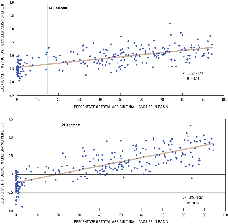
Figure 6. Total phosphorus and total nitrogen concentrations as a function of the percentage of total agriculture in the watersheds of the studied wadeable streams in Wisconsin. Computed thresholds in the response are identified by vertical lines. Linear-regression lines and coefficients of determination (R2) are given on each graph.
Concentrations of SCHL were significantly correlated with P and N concentrations (tables 4 and 5). To better define these relations, logarithmically transformed SCHL concentrations were plotted against logarithmically transformed P and N concentrations (fig. 7) and regression-tree analyses were done. Regression-tree results indicate that the best breakpoint in the response of SCHL to changes in P concentration was at 0.070 mg/L (log P = -1.16) and to changes in N concentrations occurred at 1.169 mg/L (log N = 0.07); both breakpoints were statistically significant at p < 0.001. The relations between SCHL and P and N concentrations appear linear and the regression line defines the response better than a step change in median P concentrations; however, the step-change response better defines the relation with N (on the basis of a mean-square-error criterion). A similar response was found between P and SCHL in temperate streams, with the greatest increase in SCHL occurring at P concentrations less than 0.1 mg/L (Van Nieuwenhuyse and Jones, 1996).
Table 5. Spearman correlation coefficients (rs) between residualized logarithmically transformed median concentrations of total phosphorus, dissolved phosphorus, nitrogen, nitrite plus nitrate, total Kjeldahl nitrogen, ammonia and suspended chlorophyll a, median Secchi tube depths, and specific residualized environmental (basin, soil, and surficial-deposit) characteristics for the studied wadeable streams in Wisconsin.
[PRes, residualized total phosphorus; DPRes, residualized dissolved phosphorus; NRes residualized nitrogen; NO3-NRes, residualized nitrite plus nitrate; NH4-NRes. residualized ammonia; TKNRes, residualized total Kjeldahl nitrogen; SDRes, residualized Secchi tube depth; SCHLRes, residualized suspended chlorophyll a concentration; all values with an absolute value greater than 0.18 are statistically significant at p < 0.05; all statistically significant values (not including relations between nutrients) are in bold ]
| Residualized characteristic | PRes | DPRes | NRes | NO3-N Res | NH4-N Res | TKNRes | SDRes | SCHLRes |
|---|---|---|---|---|---|---|---|---|
|
|
||||||||
| Total phosphorus | 1.00 | 0.91 | -0.02 | -0.29 | 0.58 | 0.55 | -0.26 | 0.22 |
| Dissolved phosphorus | .91 | 1.00 | .00 | -.22 | .50 | .48 | -.15 | .07 |
| Total nitrogen | -.02 | .00 | 1.00 | .55 | .09 | .01 | -.15 | -.11 |
| Dissolved nitrite plus nitrate | -.29 | -.22 | .55 | 1.00 | -.22 | -.56 | .14 | -.30 |
| Dissolved ammonia | .58 | .50 | .09 | -.22 | 1.00 | .63 | -.31 | .28 |
| Total Kjeldahl nitrogen | .55 | .48 | .01 | -.56 | .63 | 1.00 | -.25 | .40 |
| Suspended chlorophyll a | .22 | .07 | -.11 | -.30 | .28 | .40 | -.18 | 1.00 |
| Secchi tube depth | -.26 | -.15 | -.15 | .14 | -.31 | -.25 | 1.00 | -.18 |
|
|
||||||||
| Watershed area | -.18 | -.19 | -.06 | .03 | -.22 | -.05 | .09 | .14 |
| Air temperature | -.08 | -.09 | .24 | .43 | .00 | -.27 | -.06 | -.10 |
| Precipitation | -.07 | -.06 | .22 | .36 | -.12 | -.37 | -.05 | -.03 |
| Runoff | -.10 | -.08 | -.18 | -.41 | -.18 | .04 | -.07 | .03 |
| Basin slope | .01 | .07 | .01 | .33 | -.09 | -.48 | .01 | -.32 |
| Flow per unit area | -.05 | -.01 | .09 | .13 | -.06 | -.16 | .06 | -.08 |
|
|
||||||||
| Clay content | .08 | .15 | -.11 | .02 | -.04 | -.19 | -.28 | -.13 |
| Erodibility | .13 | .19 | -.09 | -.02 | -.08 | -.12 | -.02 | .00 |
| Organic-matter content | -.11 | -.16 | -.09 | -.44 | .08 | .41 | -.13 | .23 |
| Permeability | -.28 | -.34 | .06 | .01 | -.02 | .06 | .14 | .07 |
| Soil slope | -.20 | -.19 | .06 | .39 | -.23 | -.61 | .09 | -.24 |
|
|
||||||||
| Nonglacial deposits | -.18 | -.13 | .16 | .28 | -.19 | -.50 | -.02 | -.19 |
| Clay | .12 | .12 | -.27 | -.34 | .10 | .27 | -.22 | .06 |
| Loam | .12 | .11 | -.09 | -.13 | .03 | .11 | .05 | -.06 |
| Peat | .06 | .03 | .07 | -.03 | .08 | .09 | -.04 | .04 |
| Sand | .05 | -.01 | .03 | -.21 | .04 | .28 | .02 | .25 |
| Sand and gravel | -.31 | -.33 | -.01 | -.02 | -.03 | .14 | .04 | .07 |
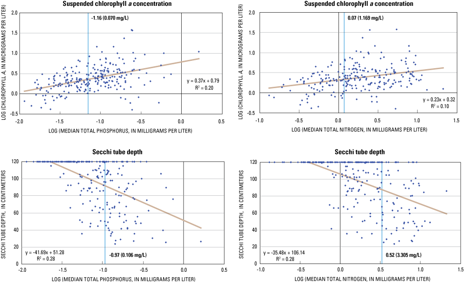
Figure 7. Suspended chlorophyll a (SCHL) concentrations and Secchi tube depths (SDs) as a function of median total phosphorus and total nitrogen concentrations (logarithm to base 10 transformation) for the studied wadeable streams in Wisconsin. Linear-regression lines and coefficients of determination (R2) are given on each graph.
To define the relations between SDs and P and N concentrations better, SDs were plotted against logarithmically transformed P and N concentrations (fig. 7) and regression-tree analyses were done. There was little apparent relation between SDs and P and between SDs and N at lower nutrient concentrations because of the limited length of the Secchi tube; however, with higher nutrient concentrations, SDs gradually decreased. Regression-tree results indicate that the best breakpoint in the response of SDs to changes in P concentrations was at 0.106 mg/L (log P = -0.97) and to changes in N concentrations was at 3.305 mg/L (log N = 0.52); both breakpoints were statistically significant at p < 0.001. A regression line defines the response better than a step change for P and N (on the basis of a mean-square-error criterion). The reduction in SDs with increasing nutrient concentrations may have been caused by other factors that are correlated to P and N concentrations, such as the clay content of the soils and surficial deposits (table 4).
Forward stepwise regressions were done with all of the environmental characteristics to determine which three environmental characteristics best described the variance in P, N, and SCHL concentrations and SDs, done with only the nonanthropogenic (natural) characteristics to determine which of these characteristics best described the variance, and done with residualized characteristics (whose correlations with anthropogenic characteristics had been removed) best described the variance in the water-quality characteristics. Models with more than three variables did not significantly increase the amount of variance explained (accumulative R2 values).
The percentage of total agriculture was the first variable incorporated into the model explaining variability in P concentrations; the second and third variables were log PtS and the percentage of loam deposits in the basin, respectively (table 6). Collectively, this model explained 56 percent of the variance in P concentrations. If the anthropogenic characteristics were omitted from the analysis, the erodibility of the soil was the first variable incorporated into the model, runoff was second, and the percentage of loam deposits was third. This model explained 44 percent of the variance. After the characteristics were adjusted to remove the anthropogenic effects, residualized loam deposits became the first variable incorporated into the model, residualized sand-and-gravel deposits was second, and residualized nonglacial deposits was third. This model collectively explained 19 percent of the variance in PRes. The difference in the amount of variance explained by the first two regression models was caused by the removal of the effects of the anthropogenic characteristics that were not correlated with other environmental characteristics in the second model. The large difference in the amount of variance explained by the last two regressions was caused by the removal of all of the effects of the anthropogenic characteristics, including the independent (direct) effects and correlated (indirect) effects on the other variables.
[all regressions were on log-transformed concentrations; r, Pearson correlation coefficient; R2, coefficient of determination for the one, two, and three variable models; Res, residualized]
| Dependent variable | First variable | Second variable | Third variable |
|---|---|---|---|
| All environmental characteristics | |||
| P | Total agriculture | Point-source loading | Loam deposits |
| r | 0.66 | 0.34 | 0.24 |
| Accumulative R2 | .44 | .51 | .56 |
| No anthropogenic characteristics | |||
| P | Erodibility | Runoff | Loam deposits |
| r | .54 | -.54 | .24 |
| Accumulative R2 | .29 | .38 | .44 |
| Residualized characteristics | |||
| PRes | LoamRes deposits | Sand-and-gravelRes deposits | NonglacialRes deposits |
| r | .30 | -.29 | -.16 |
| Accumulative R2 | .09 | .15 | .19 |
|
|
|||
| All environmental characteristics | |||
| N | Total forest | Precipitation | Agriculture (row) |
| r | -.82 | .29 | .77 |
| Accumulative R2 | .67 | .69 | .72 |
| No anthropogenic characteristics | |||
| N | Air temperature | Soil slope | Clay content of soil |
| r | .75 | -.19 | .51 |
| Accumulative R2 | .56 | .59 | .61 |
| Residualized characteristics | |||
| NRes | ClayRes deposits | Air temperatureRes | PeatRes deposits |
| r | -.35 | .25 | .16 |
| Accumulative R2 | .12 | .17 | .20 |
|
|
|||
| All environmental characteristics | |||
| SCHL | Total forest | Kjeldahl nitrogen | Watershed area |
| r | -.47 | .46 | .28 |
| Accumulative R2 | .22 | .33 | .42 |
|
No anthropogenic characteristics
|
|||
| SCHL | Kjeldahl nitrogen | Watershed area | Erodibility |
| r | .46 | .28 | .33 |
| Accumulative R2 | .21 | .30 | .41 |
|
Residualized characteristics
|
|||
| SCHLRes | Kjeldahl nitrogen | Watershed areaRes | Total phosphorus |
| r | .46 | .28 | .44 |
| Accumulative R2 | .21 | .30 | .36 |
|
All environmental characteristics |
|||
| SD | Agriculture (row) | Clay deposits | Kjeldahl nitrogen |
| r | -.55 | -.32 | -.37 |
| Accumulative R2 | .30 | .37 | .43 |
|
No anthropogenic characteristics |
|||
| SD | Total phosphorus | Clay deposits | Dissolved phosphorus |
| r | -.53 | -.32 | -.44 |
| Accumulative R2 | .28 | .36 | .44 |
|
Residualized characteristics |
|||
| SDRes | Total phosphorus | Total nitrogen | Dissolved phosphorus |
| r | -.53 | -.53 | -.44 |
| Accumulative R2 | .28 | .36 | .42 |
The percentage of total forest in the basin was the first variable incorporated into the model explaining variability in N concentrations, precipitation was the second, and the percentage of row crops in the basin was the third. Collectively, this model explained 72 percent of the variance in N concentrations. If the anthropogenic characteristics were omitted from the analysis, air temperature was the first variable, soil slope was the second, and the clay content of the soil was the third. After the characteristics were adjusted to remove the anthropogenic effects, residualized clay deposits was the first variable included in the model, residualized air temperature was the second, and residualized peat deposits was the third. This model collectively explained 20 percent of the variance in N concentrations.
For both of these constituents, removing the anthropogenic effects greatly reduced the predictability of the regression models. When the direct and indirect effects of the anthropogenic characteristics were included in the models, 56 to 72 percent of the variance could be explained with three variables; however, when all of the anthropogenic effects were removed, the models only explained about 20 percent of the variance.
To develop regression models to predict SCHL and SD, all of the water-quality characteristics and environmental characteristics (including the physical-habitat characteristics, such as shading, streambank erosion, and so on) were included. The percentage of total forest in the basin was the first variable incorporated into the model to predict SCHL, TKN was the second, and watershed area was the third. Collectively, this model explained 42 percent of the variance in SCHL concentrations. If the anthropogenic characteristics were simply omitted from the analysis, TKN was the first variable selected, watershed area was the second, and soil erodibility was the third. After the environmental characteristics were adjusted to remove the anthropogenic effects, TKN was the first variable incorporated in the model, watershed area was the second, and P was the third. This model explained 36 percent of the total variance.
The percentage of row-crop agriculture in the basin was the first variable incorporated into the model to predict SDs, percentage of clay deposits was the second, and TKN was the third. Collectively, this model explained 43 percent of the variance in SDs. When the anthropogenic characteristics were omitted, total P was the first variable incorporated into the model, the percentage of clay deposits was the second, and DP was the third. After the environmental characteristics were adjusted to remove the anthropogenic effects, total P was the first variable included in the model, total N was the second, and DP was the third. This model explained 42 percent of the total variance.
Removing the anthropogenic effects on the environmental characteristics had little effect on the predictability of the SCHL and SD models when nutrients were included in the models (second and third models). The anthropogenic characteristics were strongly correlated with nutrient concentrations, and therefore, similar predictability was obtained by including either the anthropogenic characteristics or the nutrient concentrations. The SD models that included both P concentration and percentage of clay deposits were significantly better than models that only included P concentrations.
Each of the four primary water-quality characteristics (P, N, SCHL, and SD) has been shown to be influenced by the anthropogenic characteristics and other characteristics in the watershed upstream from the assessment site. The relative importance of these factors differs for each characteristic. The relative importance of each of the general types of environmental characteristics thought to influence the distribution of overall water quality, as defined by these four water-quality characteristics, was determined by partial RDA.
In the partial RDA, the environmental characteristics were divided into three main categories: anthropogenic/land-use characteristics, soil and surficial-deposit characteristics, and basin characteristics (table 2). A two-step process was used to select four characteristics to describe each category. The characteristics initially chosen were those significantly correlated with the individual water-quality characteristics. The final characteristics within a specific category were chosen to have minimal correlations among themselves. For example, the percentage of agriculture and the percentage of forest, although both strongly correlated with water quality, were not both chosen for the anthropogenic/land-use category because they were strongly correlated to one another. The anthropogenic/land-use category was described by the percentages of total agriculture, urban, and open wetland, and the log PtS in the basin. Soils/surficial deposits were described by the clay content and organic-matter content of the soils, permeability, and erodibility. The basin characteristics were described by log (watershed area), precipitation, runoff, and basin slope. The anthropogenic/land-use characteristics category reflects the extent of human intervention—characteristics that may be altered. The soil and surficial-deposit characteristics and basin characteristics categories reflect the geological and topographical effects—characteristics that cannot be altered.
The total variance in the four water-quality characteristics was separated into five categories: 1) variance explained by the anthropogenic/land-use characteristics alone, 2) variance explained by soil and surficial-deposit characteristics alone, 3) variance explained by the basin characteristics alone, 4) variance explained by the interactions of anthropogenic/land-use, soil and surficial-deposit, and basin characteristics (joint variation that could not be assigned to a single category), and 5) variance not explained by these characteristics. Results from the partial RDA indicated that these 12 characteristics collectively explained 43 percent of the variance in water quality (P, N, SCHL, and SD; p < 0.001). Independently, the anthropogenic/land-use characteristics explained 12 percent of the explained variance (5 percent of the total variance; p < 0.001; fig. 8), the soil and surficial-deposit characteristics explained 17 percent of the explained variance (7 percent of the total variance; p < 0.001), and the basin characteristics explained 4 percent of the explained variance (2 percent of the total variance; p < 0.15). The shared contribution or interactions of all three general categories of environmental characteristics explained about 67 of the explained variance or 30 percent of the total variance. Therefore, much of the variance in water quality could not be explained by a single category of environmental characteristics.
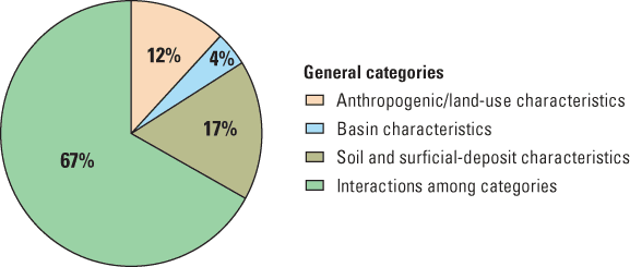
Figure 8. Percentages of explained variance in water quality (total phosphorus, total nitrogen, and suspended chlorophyll a concentrations and Secchi tube depth) described by anthropogenic/land-use, basin, soil and surficial-deposit characteristics, and interactions among categories (variance that can not be explained by a single category) for the studied wadeable streams in Wisconsin. [%, percentage of explained variance]
RDA was also used to determine which environmental characteristics explained the most variance in overall water quality (P, N, SCHL, and SD). In RDA, as in principal-component analysis, the explained variance is separated into a series of ordination (canonical) axes. Almost all of the variance in this analysis was explained on the first canonical axis. Therefore, examination of the scores on the first axis (table 7) enables the determination of the importance of individual environmental characteristics and water-quality characteristics that have the most explained variance. Total N and SD had the highest scores (absolute values) on the first canonical axis, which indicates that more of their variance was explained by the environmental characteristics than were the variances in P and SCHL. The most important characteristics explaining the variance in these four water-quality characteristics in descending order of axis score were the percentage of agriculture in the basin, the clay content of the soil, soil erodibility, runoff, and permeability. The relations between the environmental characteristics and water-quality characteristics can be determined by comparing their respective axis scores. Areas with high percentages of agriculture, high clay-content soils, highly erodible soils, low runoff, and low soil permeability had the highest nutrient and SCHL concentrations and worst water clarity. These results agree with the findings of the correlation and regression analyses.
Table 7. Results from redundancy analysis between water-quality and environmental (anthropogenic/land-use, basin, and soil and surficial-deposit) characteristics for the studied wadeable streams in Wisconsin.
[log, logarithm to base 10 transformation]
|
First canonical axis score |
|
|---|---|
| |
|
| Total phosphorus – log | 0.54 |
| Total nitrogen – log | .67 |
| Suspended chlorophyll a – log | .48 |
| Secchi tube depth | -.65 |
| |
|
| Total agriculture | .81 |
| Urban | .25 |
| Open wetland | .19 |
| Point-source loading of phosphorus – log | .31 |
| |
|
| Watershed area – log | .00 |
| Precipitation | .23 |
| Runoff | -.61 |
| Basin slope | .11 |
| |
|
| Clay content of the soil | .78 |
| Erodibility | .63 |
| Organic-matter content | -.24 |
| Permeability | -.58 |
A multiple-regression approach (similar to partial RDA) was performed to determine how the total variance in SDs and SCHL, independently, could be separated into four categories: 1) variance explained by the 5 nutrients alone (P, DP, N, NO3-N, and TKN), 2) variance explained by environmental characteristics alone (the same 12 environmental characteristics used in the partial RDA for water quality), 3) variance explained by the interactions between nutrients and environmental characteristics, and 4) variance not explained by these characteristics. In this approach, three regressions were performed for SD and for SCHL; multiple regressions with all 17 variables, with only the 5 nutrients, and with only the 12 environmental characteristics. The first regression with all 17 variables was used to determine the total variance explained by all of the variables. The other two regressions were used to partition the variance between the three categories. The amount of variance explained by the interaction of the two categories was determined by equation 10:
| EVInteractions = (EVNutrients + EVEnvironmental - EV All Variables), | (10) |
where
EV is the explained variance by the specified group of variables.
The variance explained by each subset of variables alone was then determined by subtracting the variance explained by the interactions between the variables from the total variance explained by a subset of variables. For example, the variance explained by the nutrients alone is equal to the coefficient of determination for the nutrient regression minus the variance explained by the interactions. Results from this analysis indicated that these characteristics collectively explained about 55 percent of the variance in both SDs and SCHL concentrations. Nutrients alone explained 22–23 percent of the explained variance in each of these characteristics (fig. 9). The environmental characteristics alone explained more of the variance in SCHL concentrations than in the SDs, whereas the interactions between the nutrients and environmental characteristics explained more of the variance in SDs than in SCHL concentrations. Again, much of the total variability in these two parameters could not be explained by the nutrients alone.
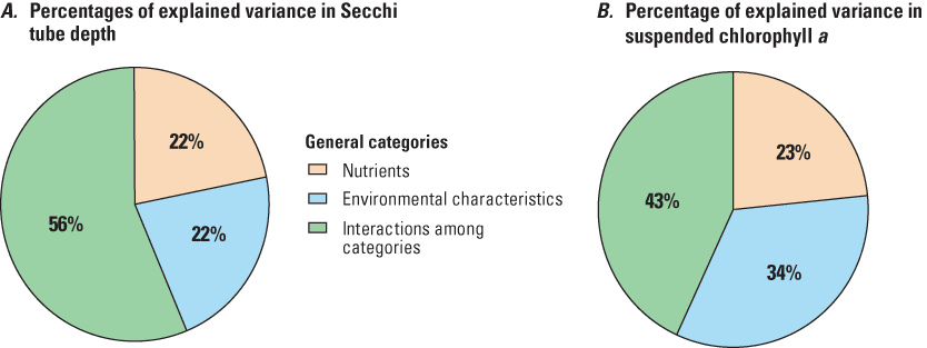
Figure 9. Percentages of explained variance in A, Secchi tube depths and B, suspended chlorophyll a concentrations described by nutrients, environmental characteristics (anthropogenic/land-use, soil, and surficial-deposit characteristics), and interactions among categories (variance that can not be explained by a single category) for the studied wadeable streams in Wisconsin. [%, percentage of explained variance]
Correlations, stepwise regressions, and regression-tree analyses all indicated that the anthropogenic/land-use characteristics (primarily the amount of forest and agriculture in the basin) were the characteristics most strongly related to water quality. Simply omitting the anthropogenic characteristics and reanalyzing the data, however, may not provide a true indication of what factors affect water quality because some of the remaining factors may be correlated with the anthropogenic characteristics of the basins. For example, air temperature and clay content of the soil were both strongly correlated with many water-quality characteristics and with the percentage of agriculture in the basin (table 4). Therefore, it is difficult to determine whether it was these factors or the indirect effects of agriculture that affected water quality. The clay content of the soil has been demonstrated to have a strong effect on the water quality of Midwestern streams (Robertson, 1997; Robertson and others, 2006); however, the effects of air temperature seem questionable and may be indirectly related to the anthropogenic characteristics.
Various approaches were used to determine which other environmental characteristics were most strongly related to water quality. The results of partial RDA indicated that soil characteristics were important; however, much of the variance explained by soil characteristics was also explained by the anthropogenic/land-use characteristics. Results of RDA indicated that the most important soil characteristics were the clay content of the soils, soil erodibility, and soil permeability. The results also indicated that the amount of runoff was also strongly related to water quality.
The results of the residualization analyses indicated that the natural (nonanthropogenic) environmental characteristics most strongly related to the distribution of P were soil permeability, the soil slope, and the percentage of sand-and-gravel deposits. The natural environmental characteristics most strongly related to the distribution of N were the percentage of clay deposits and other basin characteristics. A few of the natural characteristics, however, such as clay content of the soil and soil erodibility, were so strongly correlated with the percentage of agriculture in the basin that their relation to water quality may have been removed by the residualization approach. Stepwise regressions with residualized environmental characteristics only explained about 20 percent of the variance in P and N concentrations.
In addition to anthropogenic/land-use characteristics, residualization analyses indicated that the distribution of SCHL concentrations and SDs were related to concentrations of P and various forms of nitrogen. Other important natural characteristics related to SCHL concentrations were the slope of the basin and the soils, the organic-matter content of the soil, and some surficial-deposit characteristics. Other important natural characteristics related to SDs were the clay content of the soil and surficial deposits.
The two primary regionalization schemes considered in choosing the sites for this study and for developing nutrient criteria for Wisconsin were the level III ecoregions of Omernik and others (2000) and the environmental phosphorus zones of Robertson and others (2006) (fig. 2). In addition, a third regionalization scheme was considered after the sites were chosen and sampled. In this third scheme, the EPZs were refined based on the water-quality and environmental characteristics of only the 240 sites in this study rather than from information from sites throughout the entire upper Midwest. To refine the EPZs in figure 2B, the SPARTA approach (Robertson and others, 2006) was used with land-use-adjusted (residualized) water-quality and environmental characteristics computed for each site to remove the direct and indirect effects of land use (and PtS). P concentrations and many of the natural environmental characteristics related to P (such as the clay content of the soil and soil erodibility) were so strongly correlated with land use (and PtS) that the residualization process almost completely removed their relations with residualized P concentrations. These correlations resulted in a regionalization scheme that explained very little variance in P concentrations and which did not demonstrate clear regional patterns. Therefore, the revised EPZ regionalization scheme based on data from only the 240 sites in this study was discarded.
The primary purpose of most regionalization schemes is to minimize the variability in water quality within regions and maximize the variability among regions. This purpose was the reasoning behind the use of Omernik's ecoregions as the building block for USEPA's nutrient ecoregions. The distribution of agriculture differs among the four level III ecoregions in Wisconsin (fig. 10A). Almost 90 percent of the sites in the NLF had less than 8 percent agriculture in their basins; whereas, over 75 percent of the sites in the SWTP had over 50 percent agriculture in their basins. The use of land-use information to delineate specific regions may minimize the variability in water quality within the ecoregions across the upper Midwest and in Wisconsin because land use is the most important factor influencing the geographic distribution of most water-quality characteristics. The USEPA, however, has stated that the environmental characteristics used to delineate regions of similar reference or potential water quality should be restricted, as much as possible, to those that are intrinsic, or natural, and not the result of human activities (U.S. Environmental Protection Agency, 2000a). Therefore, the most appropriate stratification scheme for developing nutrient criteria for Wisconsin should be one that delineates areas with different reference or potential nutrient concentrations (not necessarily actual water quality), different responses in nutrient concentrations to changes in land use, and different biotic responses to changes in nutrients.
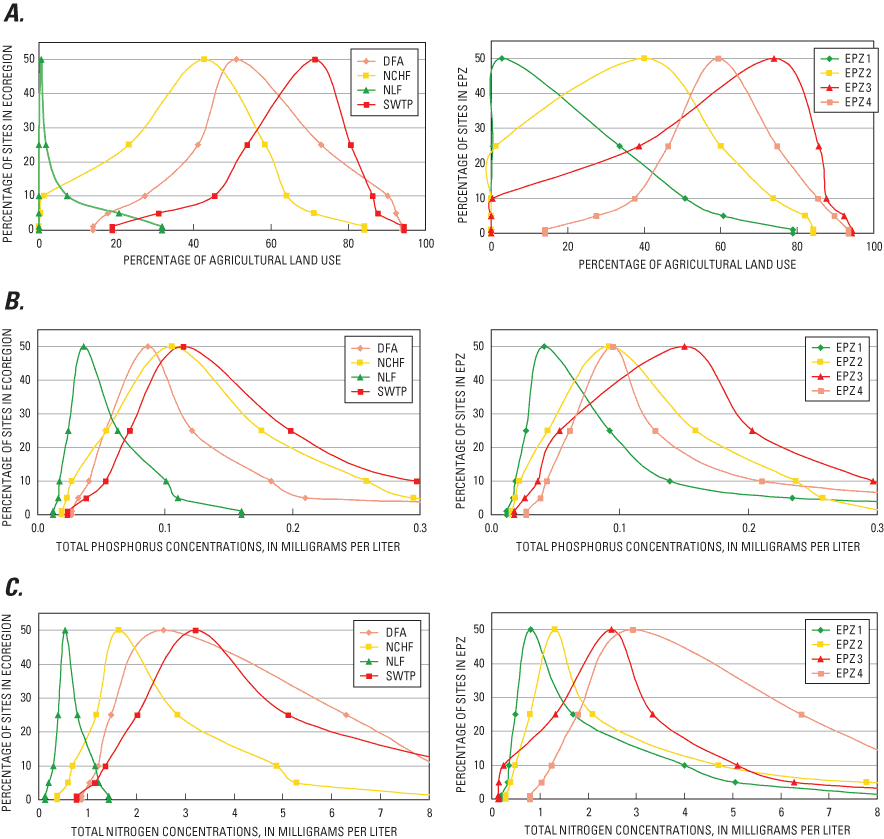
Figure 10. Percentiles of A, total agriculture in the watersheds, B, total phosphorus, and C, total nitrogen in streams in the level III ecoregions and environmental phosphorus zones (EPZs) for the studied wadeable streams in Wisconsin. [DFA, Driftless Area; NCHF, North Central Hardwood Forests; NLF, Northern Lakes and Forests; and SWTP, Southeastern Wisconsin Till Plains]
Various approaches have been used to define reference water quality for specific areas. Reference water quality is also referred to as background or potential water quality in other publications. In defining reference conditions for national nutrient criteria, the USEPA has suggested that a value based on the frequency distribution of the data available for a specific area could be used to define a reference condition. The USEPA has suggested that the value indicative of reference conditions be defined as the lower 25th percentile of all the data for that area or the upper (or worst) 75th percentile of the data for a subset of streams thought to be minimally impacted (U.S. Environmental Protection Agency, 2000a). Because it is often difficult to determine which sites are minimally impacted, the lower 25th percentile is the more common approach and the one that has been used by the USEPA to define their proposed water-quality criteria (table 1; U.S. Environmental Protection Agency, 2004).
One of the problems with the percentile approach (25th percentile) is that differences in land use within the ecoregions and zones can strongly affect the results for characteristics correlated with land use, such as the water-quality characteristics examined in this study. The reference P and N concentrations based on the percentile approach were directly related to the percentage of the sites within each ecoregion or zone dominated by agriculture. In the ecoregions examined in this study, the percentages of sites dominated by agriculture decrease from the SWTP to DFA to NCHF to NLF (fig. 10A). These differences in land use result in a gradient of conditions affecting water quality, and result in P, N, and SCHL concentrations and SDs at the 25th percentile that follow the same gradient (25th percentiles in table 8). For the EPZs, the percentages of agriculture in the basins decreased from EPZ 3 to EPZ 4 to EPZ 2 to EPZ 1, and results for the nutrient concentrations and SDs at the 25th percentile followed the same gradient except for EPZ 3 and EPZ 4, which were sometimes reversed (table 8). Therefore, the values of the water-quality characteristics at the 25th percentile do not appear to represent the true, or even relative, reference conditions for these different ecoregions and zones. The differences in the values at the 25th percentile represent the differences in the types of land uses among the different ecoregions and zones.
Table 8. Reference conditions for total phosphorus, total nitrogen, and suspended chlorophyll a concentrations, and Secchi tube depths in the environmental phosphorus zones and level III ecoregions for wadeable streams in Wisconsin. Median reference values, standard errors, and upper 95-percent confidence limits were estimated with the multiple linear-regression approach.
[USEPA, U.S. Environmental Protection Agency; EPZ, environmental phosphorus zone; DFA, driftless area; NCHF, North Central Hardwood Forests; NLF, Northern Lakes and Forests; SWTP, Southeastern Wisconsin Till Plains; --, no data; mg/L, milligram per liter; µg/L, microgram per liter; cm, centimeter; >, greater than; --, not available]
| Zone/ecoregion | Number of sites | Multiple linear-regression approach | USEPA criteria | Percentiles | ||||||||
|---|---|---|---|---|---|---|---|---|---|---|---|---|
| Median reference | Standard error | Upper 95-percent confidence limit | 0 | 10 | 25 | 50 | 75 | 90 | 100 | |||
|
|
||||||||||||
| EPZ 1 | 69 | 0.032 | 0.003 | 0.039 | -- | 0.012 | 0.019 | 0.027 | 0.041 | 0.092 | 0.139 | 0.527 |
| EPZ 2 | 58 | .042 | .006 | .054 | -- | .016 | .022 | .044 | .092 | .159 | .237 | .304 |
| EPZ 3 | 25 | .029 | .006 | .043 | -- | .018 | .036 | .053 | .150 | .203 | .297 | .741 |
| EPZ 4 | 84 | .035 | .009 | .055 | -- | .027 | .043 | .061 | .095 | .128 | .210 | 1.641 |
| DFA | 58 | .040 | .008 | .057 | .070 | .027 | .040 | .053 | .087 | .121 | .183 | .611 |
| NCHF | 48 | .041 | .009 | .060 | .029 | .019 | .027 | .054 | .106 | .176 | .258 | .527 |
| NLF | 62 | .032 | .002 | .036 | .010 | .012 | .017 | .024 | .036 | .063 | .101 | .160 |
| SWTP | 72 | .025 | .008 | .044 | .080 | .023 | .053 | .072 | .114 | .199 | .297 | 1.641 |
|
|
||||||||||||
| EPZ 1 | 69 | .557 | .057 | .676 | -- | .191 | .353 | .486 | .808 | 1.690 | 4.005 | 8.240 |
| EPZ 2 | 58 | .632 | .066 | .771 | -- | .298 | .492 | .793 | 1.303 | 2.095 | 4.710 | 21.260 |
| EPZ 3 | 25 | .367 | .103 | .601 | -- | .131 | .244 | 1.318 | 2.481 | 3.340 | 5.095 | 10.465 |
| EPZ 4 | 84 | .690 | .161 | 1.050 | -- | .780 | 1.240 | 1.780 | 2.920 | 6.420 | 8.720 | 13.205 |
| DFA | 58 | .643 | .118 | .901 | 1.880 | .882 | 1.223 | 1.489 | 2.563 | 6.300 | 8.145 | 11.385 |
| NCHF | 48 | 1.132 | .229 | 1.637 | .460 | .391 | .698 | 1.188 | 1.646 | 2.843 | 4.870 | 8.240 |
| NLF | 62 | .509 | .038 | .587 | .200 | .131 | .298 | .403 | .548 | .793 | 1.158 | 1.435 |
| SWTP | 72 | .811 | .258 | 1.409 | 1.590 | .777 | 1.361 | 2.020 | 3.204 | 5.110 | 8.720 | 21.260 |
|
|
||||||||||||
| EPZ 1 | 69 | 1.56 | 0.17 | 1.93 | -- | 0.40 | 0.65 | 1.37 | 1.95 | 2.63 | 3.97 | 14.64 |
| EPZ 2 | 58 | 1.71 | .24 | 2.23 | -- | .45 | 1.03 | 1.56 | 2.34 | 3.86 | 5.60 | 38.01 |
| EPZ 3 | 25 | 1.03 | .24 | 1.55 | -- | .77 | 1.14 | 1.62 | 2.48 | 3.80 | 7.11 | 36.63 |
| EPZ 4 | 84 | 1.17 | .25 | 1.72 | -- | .94 | 1.35 | 1.86 | 2.44 | 3.48 | 5.94 | 23.51 |
| DFA | 58 | 1.48 | .25 | 2.02 | -- | .94 | 1.35 | 1.75 | 2.16 | 2.90 | 4.12 | 14.64 |
| NCHF | 48 | 1.73 | .41 | 2.65 | -- | .40 | .74 | 1.49 | 2.43 | 3.84 | 5.78 | 7.46 |
| NLF | 62 | 1.49 | .12 | 1.74 | -- | .41 | .77 | 1.08 | 1.71 | 2.34 | 3.06 | 4.82 |
| SWTP | 72 | 1.44 | .54 | 2.71 | -- | 1.19 | 1.62 | 2.02 | 3.07 | 5.22 | 10.10 | 38.01 |
| EPZ 1 | 69 | 115.0 | 2.5 | >120.0 | -- | 35.5 | 98.0 | >120.0 | >120.0 | >120.0 | >120.0 | >120.0 |
| EPZ 2 | 58 | 117.7 | 4.9 | >120.0 | -- | 27.0 | 47.5 | 88.5 | 117.5 | >120.0 | >120.0 | >120.0 |
| EPZ 3 | 25 | 109.5 | 10.6 | >120.0 | -- | 23.5 | 42.5 | 51.5 | 76.0 | 102.5 | >120.0 | >120.0 |
| EPZ 4 | 84 | >120.0 | 10.2 | >120.0 | -- | 25.5 | 41.5 | 65.3 | 95.5 | >120.0 | >120.0 | >120.0 |
| DFA | 58 | 118.6 | 9.2 | >120.0 | -- | 35.5 | 50.0 | 67.5 | 98.0 | >120.0 | >120.0 | >120.0 |
| NCHF | 48 | 104.4 | 6.2 | 116.9 | -- | 35.5 | 81.0 | 102.3 | >120.0 | >120.0 | >120.0 | >120.0 |
| NLF | 62 | 116.5 | 1.7 | 119.8 | -- | 66.0 | 102.0 | >120.0 | >120.0 | >120.0 | >120.0 | >120.0 |
| SWTP | 72 | >120.0 | 13.4 | >120.0 | -- | 23.5 | 33.0 | 47.8 | 84.0 | 108.3 | >120.0 | >120.0 |
Another approach to estimate reference concentrations is a multiple linear-regression model that relates water quality to anthropogenic characteristics (Dodds and Oakes, 2004). After calibrating the model with data from a specific area, an estimate of reference conditions in the absence of anthropogenic activities can be obtained by setting the variables describing anthropogenic characteristics to 0 (in this study, setting percentage of agricultural area to 0, percentage of urban area to 0, and PtS to 0). These relations can also be used to place confidence intervals on the reference concentrations. Reference conditions were computed for each level III ecoregion and EPZ (fig. 2) based on all of the data available for each area with the general multiple linear-regression model:
Log PPredicted = a + b Ag% + c Urb% + d Log(PtS), (11)
where
a, b, c, and d are empirical coefficients determined for each area.
The general form of this model is similar to that used to estimate residualized concentrations in equations 3, 5, 7, and 9 (pages 24 and 25). Because this type of model estimates the logarithm of the reference concentration, the median reference concentration for each area was estimated as 10a. For each level III ecoregion and EPZ, the median reference condition, the standard error of the reference condition, and the upper bound of the 95-percent confidence interval of the reference condition were estimated (table 8). A bias correction is typically applied to results for mean values obtained by logarithmic regression; however, the bias correction was not used here because of the choice of median rather than mean reference conditions.
Reference concentrations for P ranged from 0.029 mg/L in EPZ 3 to 0.042 mg/L in EPZ 2, with the upper 95-percent confidence intervals ranging from 0.039 mg/L in EPZ 1 to 0.055 mg/L in EPZ 4 (table 8). No statistical differences are present among the reference concentrations for these zones. The regression approach was also used to estimate reference concentrations for each level III ecoregion. Reference concentrations ranged from 0.025 mg/L in the SWTP to 0.041 mg/L in the NCHF. The upper 95-percent confidence intervals ranged from 0.036 mg/L in the NLF to 0.060 mg/L in the NCHF. Again, no statistical differences are present among these concentrations. The standard errors for the reference concentrations of the EPZs were similar in magnitude to those of the ecoregions (from 0.002 to 0.009 mg/L); therefore, neither regionalization scheme was better in estimating reference P concentrations. Both regionalization schemes indicate that one reference P concentration would be appropriate for wadeable Wisconsin streams: 0.03–0.04 mg/L with an upper 95-percent confidence limit of 0.04–0.06 mg/L.
Reference concentrations for N ranged from 0.367 mg/L in EPZ 3 to 0.690 mg/L in EPZ 4, with the upper 95-percent confidence intervals ranging from 0.601 mg/L in EPZ 3 to 1.050 mg/L in EPZ 4 (table 8). Reference concentrations for EPZ 3 were lower than those for the other EPZs; however, the differences were not significant at p < 0.05. Reference concentrations ranged from 0.509 mg/L in the NLF to 1.132 mg/L in the NCHF. The upper 95-percent confidence intervals ranged from 0.587 mg/L in the NLF to 1.637 mg/L in the NCHF. Reference concentrations for the NCHF were slightly higher than those for the other ecoregions; however, no statistical differences were present between these concentrations. The standard errors of the reference concentrations of the EPZs ranged from 0.066 to 0.161 mg/L, compared to 0.038 to 0.258 mg/L for the level III ecoregions; the 95-percent confidence limits for the EPZs were generally smaller than those of the ecoregions. Therefore, the EPZs provided more precise estimates of reference N concentrations, although the differences were not significant at p < 0.05. On the basis of the EPZ regionalization scheme, two reference N concentrations may be appropriate for wadeable Wisconsin streams: 0.6–0.7 mg/L in all streams except those in EPZ 3, where 0.4 mg/L may be more appropriate.
Reference concentrations for SCHL ranged from 1.03 µg/L in EPZ 3 to 1.71 µg/L in EPZ 2, with the upper 95-percent confidence intervals ranging from 1.55 µg/L in EPZ 3 to 2.28 µg/L in EPZ 2 (table 8). Reference concentrations for EPZ 3 were lower than those for the other EPZs; however, the differences were not significant at p < 0.05. Reference concentrations ranged from 1.44 to 1.73 µg/L in the four level III ecoregions, with the upper 95-percent confidence intervals ranging from 1.74 µg/L in the NLF to 2.71 µg/L in the SWTP. Again, the differences were not significant at p < 0.05. The standard errors for the reference concentrations of the EPZs ranged from about 0.17 to 0.25 µg/L compared to 0.12 to 0.54 µg/L for the ecoregions; the 95-percent confidence limits for the EPZs were generally smaller than those of the ecoregions. Therefore, the EPZs provided more precise estimates of reference SCHL concentrations, although the differences were not significant at p < 0.05. On the basis of the EPZ regionalization scheme, two reference SCHL concentrations may be appropriate for wadeable Wisconsin streams: 1.2–1.7 µg/L in all streams except those in EPZ 3, where 1.0 µg/L may be more appropriate.
Reference SCHL concentrations and the relative importance of P and N in controlling or limiting SCHL at low nutrient concentrations was also estimated by examining the SCHL concentrations in sites with either or both reference P and reference N concentrations. For this analysis, the 240 sites were divided into five categories: reference sites (Reference, fig. 11)—36 sites with both P concentrations at or below the 0.04-mg/L reference concentration and N concentrations at or below the 0.70-mg/L reference concentration; reference P sites (Ref P)—22 sites with P concentrations at or below the reference concentration, but with N concentrations above the reference concentration; reference N sites (Ref N)—10 sites with N concentrations at or below the reference concentration, but with P concentrations above the reference concentration; high nutrient-concentration sites (High)—135 sites with both P and N concentrations above their respective upper 95-percent confidence limits for reference concentrations (P concentrations above 0.06 mg/L and N concentrations above 1.0 mg/L); and nonclassified sites—37 sites with P and N concentrations above their respective reference concentrations but below their upper 95-percent confidence limits (these sites were not included in this analysis and not included in figure 11). Comparison of the SCHL concentrations for the Reference sites with those of the Ref P and Ref N sites is similar to the comparison of SCHL concentrations for nutrient-addition experiments. SCHL concentrations for Ref P sites are similar to SCHL concentrations for experiments with N additions, and the SCHL concentrations for the Ref N sites are similar to those for experiments with P additions.
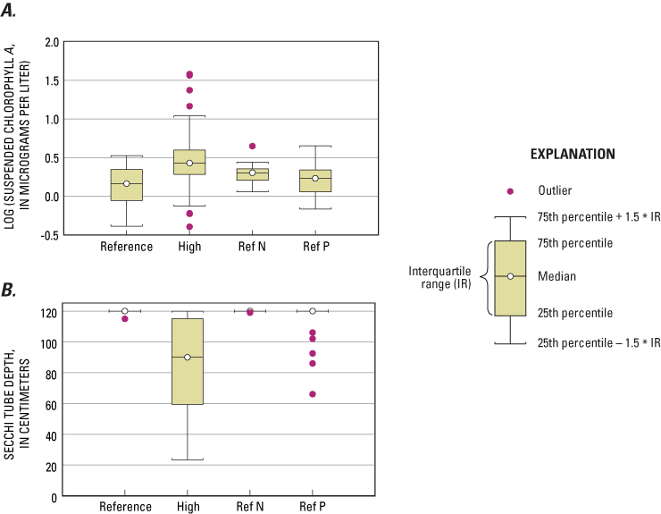
Figure 11. A, suspended chlorophyll a (SCHL) concentrations and B, Secchi tube depths (SDs) in Reference sites, High (nonreference) sites, and sites with only reference total nitrogen (Ref N sites) or reference total phosphorus (Ref P sites) concentrations in the studied wadeable streams in Wisconsin.
The approach described above was used to estimate the reference SCHL concentration for the entire State because nutrient concentrations at or below reference concentrations were primarily measured only in the northern part of the State. The median SCHL concentration of the Reference sites was 1.46 µg/L (log(1.46) = 0.16), with the upper 75th percentile being 2.22 µg/L (log(2.22) = 0.35), which was significantly less than the median concentration of 2.75 µg/L (log(2.75) = 0.44) measured in the High sites (fig. 11A). It has been suggested by the USEPA that the upper 75th percentile of a subset of streams thought to be minimally impacted (Reference sites) may represent the reference condition; therefore, an alternative reference SCHL concentration for the entire State would be 2.22 µg/L. The reference values estimated with both approaches are less than those defined by the USEPA for nutrient ecoregions 7 and 8 when the trichromatic method of analysis is used (5.8 and 4.3 µg/L, respectively; table 1).
Comparing the median concentration for the Reference sites with the median concentrations for the Ref N and Ref P sites may provide an indication of whether P or N is more important in limiting the concentrations of SCHL in streams with nutrient concentrations near reference conditions (fig. 11A). The median SCHL concentrations for Ref P and Ref N sites were both higher than that for the Reference sites, although the median concentrations for these categories were not statistically different from one another at p < 0.05. The Ref N sites had a median SCHL concentration most different from that of the Reference sites; therefore, it appears that it may be more important to have low P concentrations than low N concentrations to limit SCHL concentrations (in other words, potential P limitation for sites near reference conditions).
Reference SDs ranged from about 110 cm in EPZ 3 to greater than 120 cm in EPZ 4, with all upper 95-percent confidence intervals greater than 120 cm (table 8). These differences were not statistically different from one another at p < 0.05. Reference SDs ranged from 104.4 cm in the NCHF to greater than 120 cm in the SWTP. The upper 95-percent confidence intervals ranged from 116.9 cm in the NCHF to greater than 120 cm in the DFA and the SWTP. These differences were not statistically different from one another at p < 0.05. The standard errors of the EPZs ranged from 2.5 to 10.6 cm, compared to 1.7 to 13.4 cm for the ecoregions. Therefore, the EPZs provided slightly more precise estimates of reference clarity than the level III ecoregions, although the differences were not statistically different from one another at p < 0.05. On the basis of the EPZ regionalization scheme, two reference SDs may be appropriate for wadeable Wisconsin streams: greater than 115 cm for all streams except those in EPZ 3, where greater than 110 cm may be more appropriate.
A reference SD was also determined by examining the sites at which both P and N concentrations were at or below their respective reference concentrations. The median SD measured at the Reference sites was greater than 120 cm, which was significantly greater than the median SD measured in the High sites (90 cm; fig. 11B). The lower 25th percentile of SDs at the Reference sites (equivalent to the worst 75th percentile of the minimally impacted sites) was greater than 120 cm; therefore, an alternative reference SD for the entire State would be greater than 120 cm. The median SDs for Ref P and Ref N sites were similar to that for the Reference sites (fig. 11B); therefore, a 120-cm Secchi tube was not long enough to determine whether small increases in P or N concentrations were more important in reducing water clarity.
The responses of specific nutrients to changes in land use or other anthropogenic characteristics, such as PtS, can be estimated for each EPZ and ecoregion by the ways in which concentrations in each area change as a function of a specific anthropogenic characteristic. Overall, concentrations of P and N increase as the percentage of agricultural land increases (figs. 12A, B and 13A, B); however, variation in these responses may be associated with other anthropogenic characteristics such as differences in PtS or the percentage of urban area in the watershed. The four sites in EPZ 5 are plotted in figures 12 and 13 (and in the figures for other water-quality characteristics and biotic indices); however, these sites were not used to obtain regression lines or used in the multiple-regression analyses for P or any of the other water-quality characteristics.
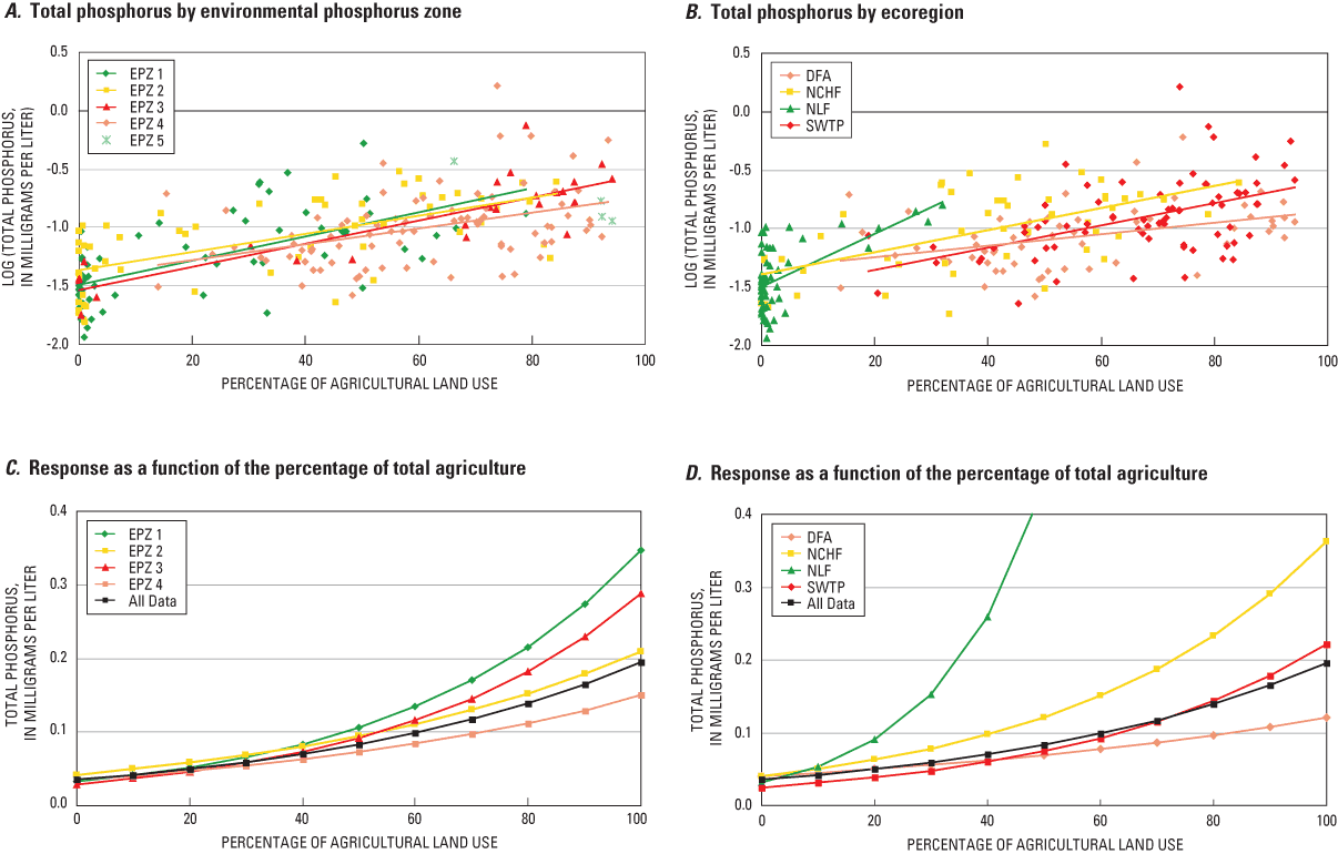
Figure 12. Total phosphorus concentrations as a function of the percentage of agricultural land use in A, environmental phosphorus zones (EPZs) and B, level III ecoregions, and response curves for phosphorus concentrations as a function of the percentage of agriculture in the watershed, in C, EPZs, and D, level III ecoregions for wadeable streams in Wisconsin. [DFA, Driftless Area; NCHF, North Central Hardwood Forests; NLF, Northern Lakes and Forests; and SWTP, Southeastern Wisconsin Till Plains]
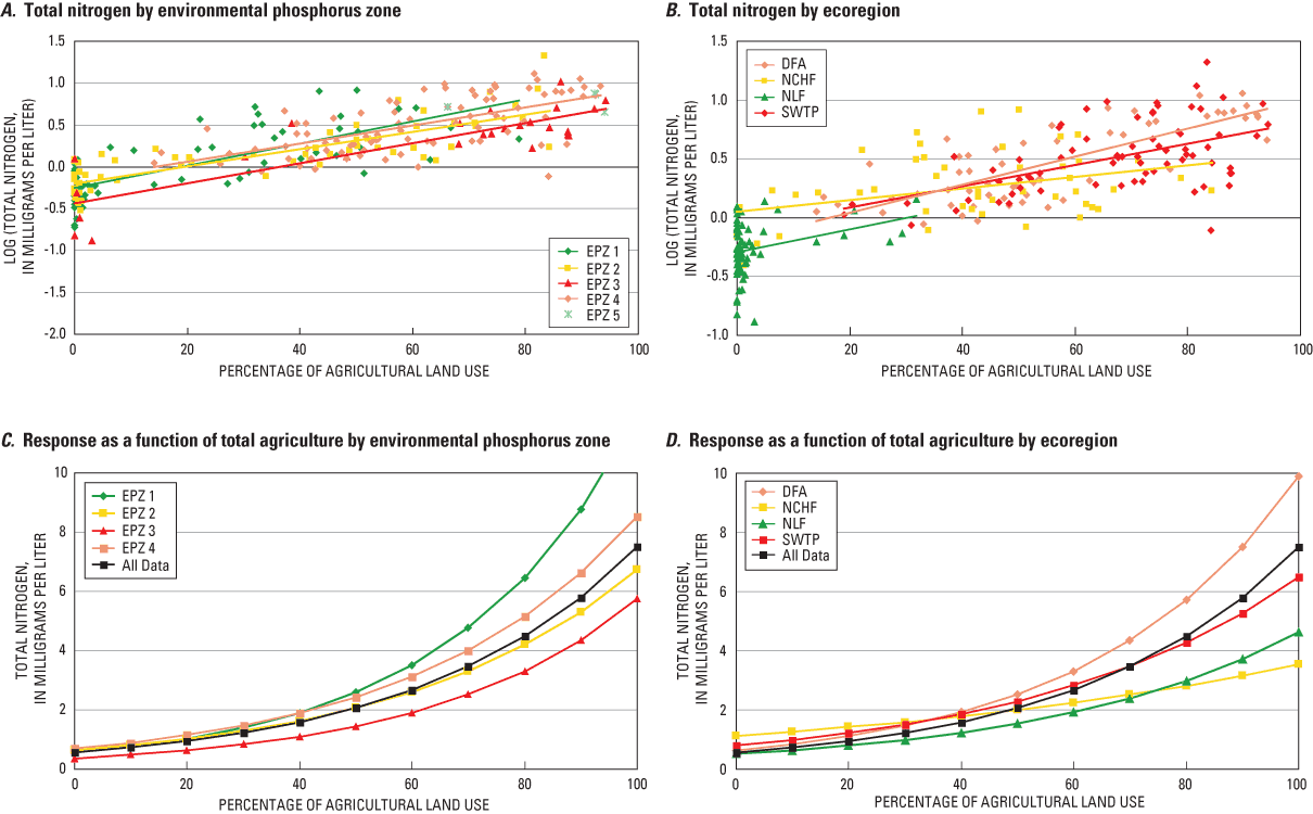
Figure 13. Total nitrogen concentrations as a function of the percentage of agricultural land use in A, environmental phosphorus zones (EPZs) and B, level III ecoregions, and response curves for nitrogen concentrations as a function of the percentage of agriculture in the watershed, in C, EPZs, and D, level III ecoregions for wadeable streams in Wisconsin. [DFA, Driftless Area; NCHF, North Central Hardwood Forests; NLF, Northern Lakes and Forests; and SWTP, Southeastern Wisconsin Till Plains]
A better approach to estimate the response of specific water-quality characteristics to changes in specific anthropogenic characteristics is the use of multiple-regression equations, such as those used to estimate reference concentrations. The response of a specific water-quality characteristic (for example, P) can be estimated for each EPZ and level III ecoregion shown in figure 2 by first determining values for the coefficients a, b, c, and d, in equation 11 on the basis of all of the available data for each zone or ecoregion. Concentrations can then be predicted as a function of specific anthropogenic characteristics by varying the characteristic of interest while holding the other characteristics constant; in this case, at 0 percent or 0 PtS (figs. 12C, D and 13C, D). This approach removes the complicating effects of the other characteristics. Because this equation estimates the logarithm of the concentration, the final concentrations were computed as 10a. A bias correction is typically applied to the results for mean values obtained by logarithmic regression; however, a bias correction was not used here because of the choice of median rather than mean concentrations.
Plots of the regression lines show that concentrations of P increase as the percentage of agricultural land increases in all of the EPZs and ecoregions (figs. 12A, B); however, a more detailed evaluation of the responses of P concentrations in the EPZs and ecoregions can be made with multiple-regression analysis. The response of P concentrations to changes in only the percentage of agricultural land was largest in EPZ 1, followed by EPZ3, EPZ 2, and EPZ 4 (fig. 12C). To determine if these responses were statistically significant from one another, the standard errors in the estimates of coefficient b were used to place 95-percent confidence limits on the estimated values (table 9). The responses in P concentrations in EPZ 1 and EPZ 3 were larger than the responses in the other EPZs, although their 95-percent confidence intervals for coefficient b slightly overlapped those of the other EPZs. Because most of the sites in EPZ 1 were in areas with limited agriculture, this difference may not reflect changes that would occur at higher percentages of agriculture. Changes in P concentrations as a function of only the percentage of agricultural land were largest in the NLF ecoregion, followed by NCHF, SWTP, and DFA (fig. 12D). The response in concentrations in the NLF was significantly larger than in any other ecoregion; however, similar to EPZ 1, the ranges in the percentage of agriculture and measured P concentrations were limited, and, therefore, this difference may simply reflect the distribution of the original data. The standard errors in the estimates of coefficient b for the EPZs ranged from 0.12 to 0.15 compared to 0.13 to 0.40 for the ecoregions. Therefore, the EPZs provided better estimates of the response to changes in the amount of agriculture than the level III ecoregions. Based on the EPZ regionalization scheme, subdividing wadeable streams in Wisconsin into two categories seems appropriate: streams in areas with high clay-content soils (EPZ 3), which respond more dramatically to changes in the amount of agriculture, and streams in the rest of the State.
Table 9. Responses to changes in the percentage of agricultural land use in the watershed. Estimated values for coefficient b for total phosphorus, total nitrogen, and suspended chlorophyll a concentrations, and Secchi tube depths in environmental phosphorus zones and level III ecoregions for wadeable streams in Wisconsin.
[b, factor associated with the percentage of agriculture in the watershed (eq. 11 in the text); mg/L, milligram per liter; µg/L, microgram per liter; cm, centimeter, EPZ, environmental phosphorus zone; DFA, Driftless Area; NCHF, North Central Hardwood Forests; NLF, Northern Lakes and Forests; SWTP, Southeastern Wisconsin Till Plains]
| Zone/ecoregion | Estimated value for b | Standard error for b | Upper 95-percent confidence value for b |
|---|---|---|---|
|
|
|||
| EPZ 1 | 1.03 | 0.15 | 1.33 |
| EPZ 2 | 0.70 | .13 | 0.96 |
| EPZ 3 | .99 | .12 | 1.23 |
| EPZ 4 | .63 | .15 | .93 |
| DFA | .48 | .13 | .74 |
| NCHF | .95 | .19 | 1.33 |
| NLF | 2.28 | .40 | 3.08 |
| SWTP | .95 | .18 | 1.31 |
|
|
|||
| EPZ 1 | 1.33 | .14 | 1.61 |
| EPZ 2 | 1.03 | .10 | 1.23 |
| EPZ 3 | 1.19 | .16 | 1.51 |
| EPZ 4 | 1.09 | .14 | 1.37 |
| DFA | 1.19 | .12 | 1.43 |
| NCHF | .49 | .18 | .85 |
| NLF | .96 | .40 | 1.76 |
| SWTP | .90 | .17 | 1.24 |
|
|
|||
| EPZ 1 | .22 | .16 | .55 |
| EPZ 2 | .36 | .14 | .63 |
| EPZ 3 | .60 | .13 | .87 |
| EPZ 4 | .54 | .13 | .80 |
| DFA | .35 | .35 | 1.05 |
| NCHF | .16 | .20 | .55 |
| NLF | .93 | .44 | 1.80 |
| SWTP | .47 | .20 | .86 |
|
|
|||
| EPZ 1 | -7.1 | 8.7 | 10.3 |
| EPZ 2 | -49.8 | 11.0 | -27.8 |
| EPZ 3 | -53.0 | 15.4 | -22.1 |
| EPZ 4 | -48.5 | 16.1 | -16.2 |
| DFA | -42.1 | 15.2 | -11.8 |
| NCHF | 8.8 | 13.7 | 36.2 |
| NLF | -33.8 | 21.5 | 9.3 |
| SWTP | -89.0 | 19.2 | -50.5 |
Concentrations of N also increase as the percentage of agricultural land increases in all of the EPZs and ecoregions (fig. 13). The responses in concentrations in EPZ 1 and EPZ 4 were larger than the responses in the other EPZs, and the response in concentrations in EPZ 3 was smaller than those in the other EPZs; however, these differences were not statistically significant at p < 0.05. The changes in N concentrations were largest in the DFA, followed by SWTP, NLF, and NCHF. The response in concentrations in the DFA was significantly larger than in the NCHF, but not significantly larger than in the other ecoregions at p < 0.05. The response in concentrations in EPZ 1 was larger than in any other EPZ and the response in NLF was smaller than in any other ecoregion; however, this difference may simply reflect the distribution of the original data. The standard errors in the estimates of coefficient b for the EPZs ranged from 0.10 to 0.16 compared to 0.12 to 0.40 for the ecoregions (table 9). Therefore, the EPZs provided better estimates of the response to changes in the percentage of agricultural land use than the level III ecoregions. Based on the EPZ regionalization scheme, subdividing wadeable streams in Wisconsin into two categories seems appropriate: streams in areas with clay soils (EPZ 3), which respond less dramatically to changes in the amount of agriculture, and streams in the rest of the State.
Concentrations of SCHL increased as P and N concentrations increased; however, there was much variation in these relations (fig. 14). For any nutrient concentration, there was about an order of magnitude of variation in SCHL concentrations. Although nutrient concentrations were lower or higher in some areas (especially lower in EPZ 1 and the NLF ecoregion), there was a relatively similar response in SCHL concentrations to changes in nutrient concentrations in all EPZs and level III ecoregions. Five sites, however, had SCHL concentrations that were lower than might be expected for the measured P and N concentrations at the site. These sites were in EPZ 1 and the NCHF, and were generally small sites (5.8–55.6 km2) with extensive sedimentation and embedded rocky substrate (94–100 percent).
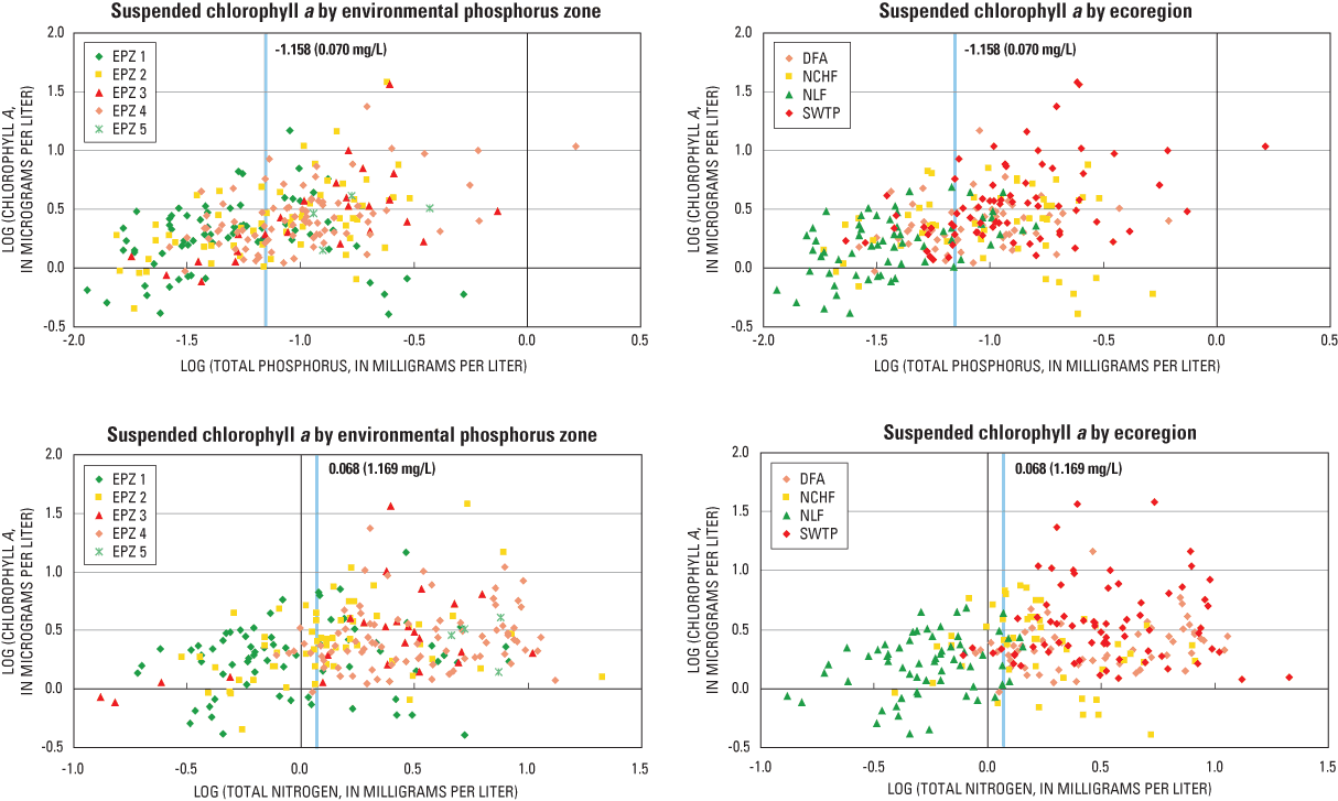
Figure 14. Suspended chlorophyll a concentrations as a function of total phosphorus and total nitrogen concentration (logarithm to base 10 transformation), by environmental phosphorus zones (EPZs) and by level III ecoregions for the studied wadeable streams in Wisconsin. Computed thresholds in the response are identified by vertical lines. [DFA, Driftless Area; NCHF, North Central Hardwood Forests; NLF, Northern Lakes and Forests; and SWTP, Southeastern Wisconsin Till Plains]
The best breakpoints or thresholds in the response of SCHL to changes in P and N concentrations were at 0.070 mg/L (log(P) = -1.16) and 1.169 mg/L (log(N) = 0.07), respectively. This P concentration is expected to occur at approximately 30- to 50-percent agriculture in all areas (fig. 12). This N concentration is expected to occur at approximately 30-percent agriculture in all areas except EPZ 3, where it occurs at about 50-percent agriculture (fig. 13).
Water clarity (SDs) decreased as P and N concentrations increased (fig. 15). At low nutrient concentrations, water clarity often exceeded the 120-cm length of the Secchi tube. Then, as nutrient concentrations increased, water clarity decreased; however, there was much variation in this relation. For most nutrient concentrations, other than very low concentrations, SDs ranged from 20 cm to greater than 120 cm. In general, the SD responses were similar in most EPZs and ecoregions. The best breakpoints or thresholds in the response of SDs to changes in P and N concentrations were at 0.106 mg/L (log(P) = -0.97) and 3.305 mg/L (log(N) = 0.52), respectively. This P concentration is expected to occur at approximately 50- to 70-percent agriculture in all areas (fig. 12). This N concentration is expected to occur at approximately 55- to 70-percent agriculture in all areas except EPZ 3, where it occurs at about 80-percent agriculture (fig. 13).
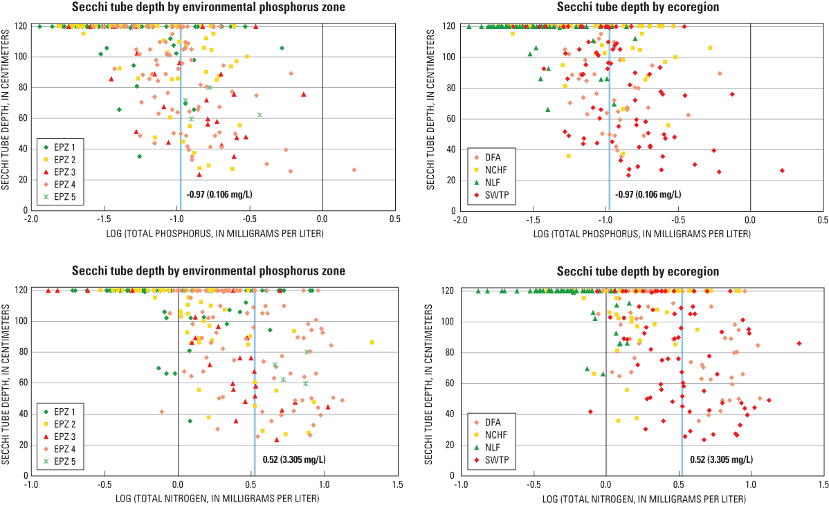
Figure 15. Secchi tube depth as a function of total phosphorus and total nitrogen concentration (logarithm to base 10 transformation), by environmental phosphorus zones (EPZs) and by level III ecoregions for the studied wadeable streams in Wisconsin. Computed thresholds in the response are identified by vertical lines. [DFA, Driftless Area; NCHF, North Central Hardwood Forests; NLF, Northern Lakes and Forests; and SWTP, Southeastern Wisconsin Till Plains]
The multiple-regression approach was again used to estimate changes in SCHL concentrations and SDs in response to changes in the percentage of agricultural land in the watershed. Concentrations of SCHL increased as the percentage of agricultural land increased in all of the EPZs (fig. 16A) and ecoregions (not shown), and the response was similar in all areas except EPZ 1. The response in concentrations in EPZ 1 was less than in any other EPZ; however, this difference may simply reflect the limited distribution of the original data in EPZ 1. The standard errors in the estimates of coefficient b for the EPZs ranged from 0.13 to 0.16 compared to 0.20 to 0.44 for the level III ecoregions (table 9). As are result, the 95-percent confidence intervals for the EPZs were smaller than those for the ecoregions. Therefore, the EPZs provided better estimates of the response in SCHL concentrations to changes in the amount of agricultural land in the watershed than the level III ecoregions. Based on the similarity in the distribution of concentrations (fig. 15) and insignificant differences in values for coefficient b among EPZs, it is not appropriate to subdivide the wadeable streams of Wisconsin based on the response in SCHL concentrations to changes in nutrient concentrations and land use.
Water clarity decreased as the percentage of agriculture land increased in all of the EPZs and level III ecoregions, and the response was similar in all areas except EPZ 1 (fig. 16B, shown for EPZs only). The water clarity decreased more slowly in EPZ 1 than in the other zones; however, there were only a few sites in EPZ 1 with extensive agriculture to support this conclusion. The response in water clarity in EPZ 3 was similar to the other areas; the difference in the water clarity in this area was caused by the lower reference clarity. The standard errors in the estimates of coefficient b for the EPZs ranged from 8.7 to 16.1 compared to 13.7 to 21.5 cm for the ecoregions (table 9). Therefore, the EPZs provided better estimates of the response in SDs to changes in the amount of agricultural land in the watershed than the level III ecoregions. Based on the results for the EPZ regionalization scheme, subdividing wadeable streams into two categories seems appropriate: streams in areas with high clay-content soils (EPZ 3), which have a lower reference water clarity and clarity that decreases and remains lower than sites in the other areas as the percentage of agricultural land in the watershed increases, and streams in the rest of the State.
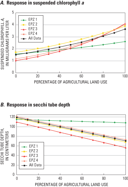
Figure 16. Response curves for A, suspended chlorophyll a concentrations and B, Secchi tube depths in the environmental phosphorus zones (EPZs) as a function of the percentage of agriculture in the watershed for wadeable streams in Wisconsin.
The streams examined in this study exhibit considerable variation in their physical habitats, particularly with respect to mean stream widths and depths. Mean widths ranged from 1.1 m to over 55 m, with an overall mean width of 7.6 m (table 10). Mean depths ranged from 0.1 m to 1.0 m, with an overall mean depth of 0.3 m. Mean thalweg depths (deepest part of the cross section) ranged from 0.1 m to 1.3 m, with an overall mean depth of 0.4 m. The gradients of the streams at the sampling sites ranged from nearly flat (0.0 m/km) to quite steep (up to 20.7 m/km) and their sinuosity (not in table 10) ranged from highly meandered to straight channels. About half of the streams contained well-developed runs. On average, 75 percent of the stream's reach was classified as runs. Most streams had less than 10 percent of the reach classified as pools and riffles. Stream bottoms ranged from being almost completely silt to being dominated by sand or gravel. The percentage of the stream's reach that was shaded ranged from 0 to 93.7 percent.
Table 10. Summary statistics for the physical-habitat characteristics and biotic indices for the studied wadeable streams in Wisconsin.
[EPT, Ephemeroptera, Plecoptera, and Trichoptera; #, number; m, meter; m/km, meter per kilometer; mg/m2, milligram per square meter; log, logarithm to base 10 transformation; --, values are not indicative of water quality]
| Characteristic/index | Abbreviation | Units | Transformation | Count | Median | Mean | Best 25th percentile of all sites | Standard deviation | Minimum | Maximum |
|---|---|---|---|---|---|---|---|---|---|---|
|
|
||||||||||
| Stream width | WIDTH | m | none | 235 | 4.5 | 7.6 | -- | 8.3 | 1.1 | 56.3 |
| Stream mean depth | DEPTH | m | none | 235 | .3 | .3 | -- | .2 | .1 | 1.0 |
| Mean thalweg depth | THALD | m | none | 235 | .4 | .4 | -- | .2 | .1 | 1.3 |
| Stream gradient | GRAD | m/km | none | 231 | 2.5 | 3.2 | -- | 3.0 | .0 | 20.7 |
| Percentage of pools | POOL% | % | none | 234 | 5.0 | 10.5 | -- | 13.9 | .0 | 100.0 |
| Percentage of riffle | RIFF% | % | none | 234 | 8.5 | 13.9 | -- | 17.2 | .0 | 100.0 |
| Percentage of run | RUN% | % | none | 234 | 49.7 | 75.3 | -- | 22.9 | .0 | 100.0 |
| Depth of sediment on stream bottom | SEDEP | m | none | 235 | .1 | .1 | -- | .1 | .0 | 0.9 |
| Percentage of silt in bottom sediments | SILT% | % | none | 235 | 10.6 | 17.2 | -- | 18.3 | .0 | 95.6 |
| Percentage of sand in bottom sediments | SAND% | % | none | 235 | 27.3 | 34.3 | -- | 25.3 | .0 | 99.6 |
| Percentage of gravel in bottom sediments | GRAV% | % | none | 235 | 18.8 | 19.6 | -- | 14.5 | .0 | 66.2 |
| Percentage of rocky-substrate embeddedness | EMB% | % | none | 235 | 64.2 | 59.8 | -- | 29.5 | 6.2 | 100.0 |
| Percentage of stream bottom covered by algae | ALGAE% | % | none | 235 | .4 | 4.8 | -- | 9.1 | .0 | 53.8 |
| Percentage of stream bottom covered by macrophytes | MACR% | % | none | 235 | 1.3 | 6.3 | -- | 10.9 | .0 | 54.8 |
| Percentage of stream with fish cover | COVER% | % | none | 235 | 7.2 | 9.3 | -- | 9.2 | .0 | 65.5 |
| Percentage of stream shaded | SHADE% | % | none | 235 | 28.9 | 33.9 | -- | 27.8 | .0 | 93.7 |
| Percentage of stream bank with erosion | EROSION% | % | none | 235 | 12.5 | 17.7 | -- | 15.9 | .0 | 76.5 |
| Buffer width | BUFFER | m | none | 235 | 10.5 | 12.6 | -- | 6.5 | .0 | 30.0 |
|
|
||||||||||
| Benthic chlorophyll a | BCHL | mg/m2 | log | 199 | 1,919 | 12,879 | 552 | 80,884 | 7 | 1,068,000 |
| Diatom Nutrient Index | DNI | # | none | 214 | 4.1 | 3.9 | 3.5 | 0.8 | 1.7 | 5.4 |
| Diatom Siltation Index | DSI | # | none | 214 | 38.2 | 39.9 | 16.7 | 24.9 | 2.6 | 95.3 |
| Diatom Biotic Index | DBI | # | none | 214 | 42.1 | 46.4 | 51.3 | 15.7 | 22.8 | 100.0 |
|
|
||||||||||
| Hilsenhoff Biotic Index | HBI | # | none | 227 | 4.7 | 4.9 | 4.0 | 1.6 | 0.8 | 9.4 |
| Percentage of EPT individuals | EPTN% | % | none | 227 | 42.3 | 41.0 | 61.8 | 26.1 | .0 | 99.2 |
| Percentage of EPT taxa | EPTTX% | % | none | 227 | 35.7 | 33.9 | 45.7 | 16.8 | .0 | 74.3 |
| Percentage of scrapers | SCRAP% | % | none | 227 | 14.7 | 19.0 | 29.5 | 18.0 | .0 | 85.4 |
| Percentage of shredders | SHRED% | % | none | 227 | 0.0 | 1.0 | -- | 3.1 | .0 | 24.7 |
| Number of taxa | TAXAN | # | none | 232 | 29 | 29.2 | 35.0 | 10.4 | 4 | 67 |
|
|
||||||||||
| Fish Index of Biotic Integrity | IBI | # | none | 235 | 40.0 | 40.2 | 52.0 | 20.8 | .0 | 100.0 |
| Percentage of carnivores | CARN% | % | none | 234 | 1.6 | 11.4 | 9.8 | 21.3 | .0 | 100.0 |
| Percentage of insectivores | INSECT% | % | none | 234 | 48.9 | 49.8 | 29.1 | 24.2 | .0 | 100.0 |
| Percentage of omnivores | OMNI% | % | none | 234 | 10.5 | 15.4 | 3.8 | 16.0 | .0 | 81.1 |
| Percentage of intolerant species | TOL% | % | none | 234 | 3.3 | 14.6 | 15.8 | 23.3 | .0 | 97.9 |
| Percentage of tolerant species | INTOL% | % | none | 234 | 42.8 | 41.5 | 19.5 | 25.6 | .0 | 100.0 |
| Number of fish | FISHN | # | log | 234 | 130 | 199.6 | -- | 247.8 | 7 | 2,147 |
| Number of fish species | FISHSPEC | # | none | 235 | 11 | 11.5 | -- | 5.4 | 1 | 33 |
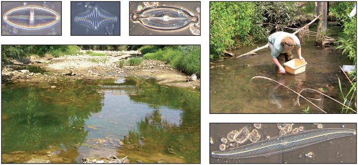 |
| Wisconsin Department of Natural Resources personnel collecting diatom samples. Microscopic diatom pictures provided by Paul Garrison (Wisconsin Department of Natural Resources). |
Four indices were used to describe the benthic chlorophyll a and periphytic-diatom communities found in the streams in this study (table 10). Benthic chlorophyll a (BCHL) concentrations ranged from 7 mg/m 2 to over 1,000,000 mg/m2 (median = 1,919 mg/m2), the Diatom Nutrient Index (DNI) values ranged from 1.7 to 5.4 (median = 4.1), the Diatom Siltation Index (DSI) values ranged from 2.6 to 95.3 (median = 38.2), and Diatom Biotic Index (DBI) values ranged from 22.8 to 100 (median = 42.1). In general, streams in the northern part of the State had lower BCHL concentrations and better quality diatom communities, lower DNI and DSI values, and higher DBI values than streams in the rest of the State (fig. 17).
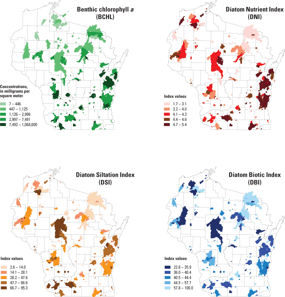
Figure 17. Distributions (quintiles) of benthic chlorophyll a (BCHL) concentrations, Diatom Nutrient Index (DNI) values, Diatom Siltation Index (DSI) values, and Diatom Biotic Index (DBI) values for the studied wadeable streams in Wisconsin.
Spearman rank correlation coefficients (rs values) between the four indices describing BCHL and diatom communities and the water-quality, environmental, and physical-habitat characteristics are given in table 11. All four indices were significantly correlated with P and DP concentrations; however, only BCHL, DNI, and DSI were significantly correlated with N and NO3-N concentrations. Only DNI and DSI were correlated with NH4-N, and only DNI was significantly correlated with TKN. The relations found for N were primarily the result of variability in NO3-N concentrations, because N was computed as the sum of NO3-N and TKN, and TKN was only weakly correlated with most indices. DSI values were more strongly correlated with nutrient concentrations than were the DNI values except for TKN, and both indices were more strongly correlated with nutrient concentrations than were DBI values. BCHL concentrations were more strongly correlated with the different forms of N, whereas the diatom indices were more strongly correlated with the different forms of P. Other studies have found the P-chlorophyll relation to be stronger than the N-chlorophyll relation (for example, Van Nieuwenhuyse and Jones, 1996).
Table 11. Spearman rank correlation coefficients (rs) between benthic chlorophyll a concentrations (BCHL) and diatom community indices, and median water-quality, environmental (anthropogenic/land-use, basin, soil and surficial-deposit), and physical-habitat characteristics for the studied wadeable streams in Wisconsin.
[all bold values were significant at p < 0.05, after being adjusted for the Bonferroni correction (Zar, 1999); see table 10 for definitions of abbreviations and units for each characteristic]
| Total phosphorus | 0.33 | 0.47 | 0.60 | -0.46 |
| Dissolved phosphorus | .33 | .47 | .59 | -.46 |
| Total nitrogen | .49 | .36 | .43 | -.10 |
| Dissolved nitrite plus nitrate | .53 | .31 | .40 | -.05 |
| Dissolved ammonia | .12 | .21 | .30 | -.13 |
| Total Kjeldahl nitrogen | -.07 | .24 | .09 | -.17 |
| Suspended chlorophyll a | .21 | .24 | .29 | -.17 |
| Secchi tube depth | -.22 | -.39 | -.41 | .17 |
| Urban | .25 | .26 | .10 | .03 |
| Agriculture (row crops) | .44 | .42 | .42 | -.13 |
| Agriculture (all) | .50 | .44 | .51 | -.14 |
| Grassland | .10 | .12 | .20 | -.14 |
| Wetland (open) | -.12 | .18 | -.22 | -.02 |
| Wetland (forested) | -.44 | -.18 | -.51 | .10 |
| Forest (all) | -.44 | -.45 | -.48 | .17 |
| Point-source loading of phosphorus | .27 | .26 | .18 | -.17 |
| Watershed area | .10 | .12 | -.07 | -.07 |
| Air temperature | .48 | .42 | .51 | .00 |
| Precipitation | .21 | .05 | .28 | .08 |
| Runoff | -.42 | -.41 | -.35 | .00 |
| Basin slope | .28 | .08 | .48 | -.15 |
| Flow per unit area | -.16 | -.17 | -.18 | .15 |
| Clay content | .46 | .44 | .63 | -.15 |
| Erodibility | .37 | .37 | .52 | -.12 |
| Organic-matter content | -.41 | -.14 | -.55 | .17 |
| Permeability | -.35 | -.36 | -.60 | .25 |
| Soil slope | .06 | -.25 | .11 | .08 |
| Nonglacial deposits | .42 | -.01 | .45 | .03 |
| Clay deposits | .10 | .30 | .13 | -.17 |
| Loam deposits | -.06 | .02 | .04 | -.25 |
| Peat deposits | -.09 | -.10 | -.05 | -.02 |
| Sand deposits | -.35 | .00 | -.34 | .12 |
| Sand-and-gravel deposits | -.26 | -.20 | -.52 | .24 |
| WIDTH | -0.03 | -0.01 | -0.17 | -0.04 |
| DEPTH | .11 | .00 | .03 | -.03 |
| THALD | .07 | -.03 | .01 | -.03 |
| GRAD | .02 | -.05 | .13 | .01 |
| POOL% | .00 | -.04 | .13 | -.02 |
| RIFF% | .13 | .13 | .11 | -.01 |
| RUN% | -.07 | -.04 | -.15 | .05 |
| SEDEP | -.04 | -.10 | -.05 | .01 |
| SILT% | .17 | .05 | .18 | .06 |
| SAND% | -.29 | -.18 | -.22 | -.02 |
| GRAV% | .00 | .22 | -.02 | -.04 |
| EMB% | -.08 | -.18 | -.06 | .04 |
| ALGAE% | .28 | .21 | .24 | .02 |
| MACR% | .01 | -.12 | -.06 | .12 |
| COVER% | -.12 | -.10 | -.19 | .06 |
| SHADE% | -.07 | .07 | -.11 | .00 |
| EROSION% | .18 | .20 | .32 | -.15 |
| BUFFER | -.03 | .09 | -.07 | .04 |
BCHL, DNI, and DSI were strongly correlated with SCHL, SD, and many of the anthropogenic/land-use characteristics, especially the percentages of total agriculture, row-crop agriculture, and forested areas. In addition, BCHL and the DNI were significantly correlated with the amount of urban land and PtS in the basin. Better index values (lower values for BCHL, DNI, and DSI) generally occurred in streams with lower SCHL and higher clarity, in areas with lower percentages of agriculture, less PtS, and higher percentages of forest. In general, these indices were also strongly correlated with several basin (air temperature and runoff) and soil (clay content, erodibility, organic-matter content, and permeability) characteristics. Lower BCHL concentrations and better diatom indices generally occurred in areas with cooler air temperatures, higher runoff, less erodible soils with lower clay content and higher permeability, and sand-and-gravel surficial deposits. These areas with lower BCHL concentrations and better diatom indices are the mixed and mostly forested areas of Wisconsin (fig. 2A).
In general, the BCHL and diatom indices were only weakly correlated with any physical-habitat characteristics except the percentage of the bottom covered in algae and the amount of sandy sediment. Better benthic diatom communities occurred in streams with lower percentages of algal cover. BCHL and the diatom indices were unrelated to the size or depth of the streams.
Responses in BCHL, DNI, and DSI to changes in nutrient concentrations are shown in figures 18 and 19 (DBI values, which were computed on the basis of DNI and DSI values, were less strongly correlated with nutrient concentrations and therefore are not shown). In general, all three indices increased as nutrient concentrations increased, although the responses to changes in N concentrations ranged more widely than changes in P. At low nutrient concentrations, the values of the indices ranged widely; however, at high nutrient concentrations, the values were generally limited to high BCHL and poor diatom indices. High BCHL concentrations and poor diatom indices were measured even at low nutrient concentrations. The lower bounds of the BCHL and DNI plots may provide an indication of the extent to which nutrients are capable of limiting BCHL and the diatom community. The variation above these bounds may indicate the effects caused by factors other than nutrients.
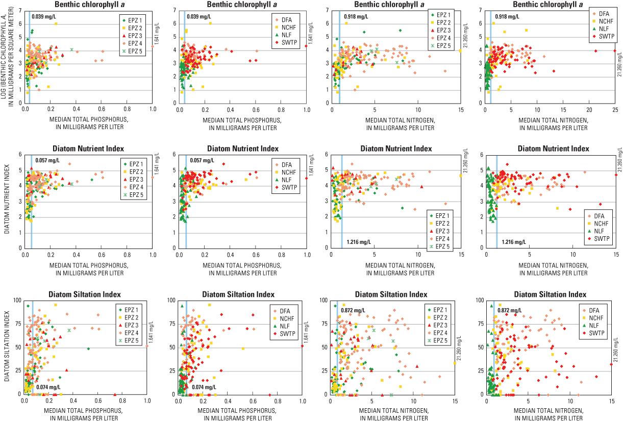
Figure 18. Benthic chlorophyll a concentrations (logarithm to base 10 transformation), Diatom Nutrient Index values, and Diatom Siltation Index values as a function of total phosphorus and total nitrogen concentration in the environmental phosphorus zones (EPZs) and level III ecoregions for the studied wadeable streams in Wisconsin. Computed thresholds in the response are identified by vertical lines. [DFA, Driftless Area; NCHF, North Central Hardwood Forests; NLF, Northern Lakes and Forests; and SWTP, Southeastern Wisconsin Till Plains]
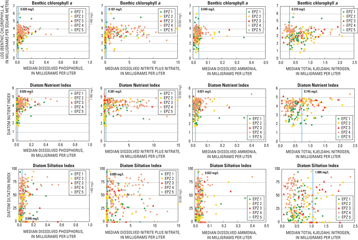
Figure 19. Benthic chlorophyll a concentrations (logarithm to base 10 transformation), Diatom Nutrient Index values, and Diatom Siltation Index values as a function of dissolved phosphorus, dissolved nitrite plus nitrate, dissolved ammonia, and total Kjeldahl nitrogen concentrations in the environmental phosphorus zones (EPZs) for the studied wadeable streams in Wisconsin. Computed thresholds in the response are identified by vertical lines.
Although nutrient concentrations were lower or higher in some EPZs and level III ecoregions (especially lower in EPZ 1 and the NLF ecoregion), BCHL concentrations and diatom indices responded similarly to changes in nutrient concentrations in all areas (fig. 18). In all EPZs and ecoregions, there was a broad response at low nutrient concentrations and poor (higher) indices at high nutrient concentrations. Differences in the responses among areas could not be distinguished because of the range in the data and because the gradient in nutrient concentrations within many areas was small.
Regression-tree analyses were done to define specific thresholds or breakpoints in the responses of BCHL concentrations and the diatom indices (table 12). The best statistical thresholds or breakpoints in the responses to changes in total P concentrations ranged from 0.039 mg/L for BCHL concentrations to 0.057–0.074 mg/L for the diatom indices. Thresholds in the response to changes in DP concentrations ranged from 0.020 mg/L for BCHL to 0.046 mg/L for DSI. Thresholds in the responses to changes in the different forms of N are also listed in table 12; however, the data in figures 18 and 19 do not show any consistent response except the DNI as a function of N. Thresholds in the responses to changes in N concentrations ranged from 0.872 to 1.216 mg/L. In general, sites with concentrations below the defined thresholds had a broad range in index values and sites above the defined threshold had poor index values, although the data do not indicate well-defined thresholds.
Table 12. Thresholds or breakpoints in the responses of benthic chlorophyll a (BCHL) concentrations and diatom indices to changes in nutrient concentrations for wadeable streams in Wisconsin.
[all nutrient concentrations are in milligrams per liter; log, logarithm to base 10 transformation]
| Biological Indices | Total phosphorus | Dissolved phosphorus | Total nitrogen | Dissolved nitrite plus nitrate | Dissolved ammonia | Total Kjeldahl nitrogen |
|---|---|---|---|---|---|---|
| Benthic chlorophyll a (BCHL) - log | 0.039 | 0.020 | 0.918 | 0.187 | 0.040 | 0.310 |
| Diatom Nutrient Index (DNI) | .057 | .026 | 1.216 | .381 | .021 | .745 |
| Diatom Siltation Index (DSI) | .074 | .046 | .872 | .089 | .022 | 1.080 |
| Diatom Biotic Index (DBI) | .072 | .039 | 1.169 | .381 | .022 | .388 |
To examine further the thresholds or breakpoints in the responses of BCHL and the diatom indices to changes in nutrient concentrations, a categorical approach developed by the Ohio Environmental Protection Agency (OEPA; Miltner and Rankin, 1998) was used to examine the BCHL and DNI responses. With this approach, not only was the response to a single nutrient constituent examined but also the interaction of P and N. For this analysis, each of the sites having BCHL and diatom index data was placed into one of five categories based upon their percentile rankings for P and N concentrations (25th, 50th, 75th, and 90th percentiles; table 13). The five categories in increasing nutrient concentrations are: category 1, sites that have both P and N concentrations less than their 25th percentiles; category 2, sites that are not in category 1 and have either P or N concentrations less than their 50th percentiles; category 3, sites that are not in categories 1 or 2 and have P concentrations less than its 75th percentile and N concentrations less than its 90th percentile; category 4, sites that are not in categories 1, 2, or 3 and have P concentrations between and including its 75th and 90th percentiles (N concentrations do not matter); and category 5, sites that have both P and N concentrations greater than their 90th percentiles (OEPA also includes a sixth category for sites that have NH4-N concentrations greater than 1.0 mg/L but there were no such sites in this study.)
Table 13. Percentiles of total phosphorus and total nitrogen concentration for the studied wadeable streams in Wisconsin having both benthic chlorophyll a and diatom index data.
[all concentrations in milligrams per liter]
| Percentile | Total phosphorus | Total nitrogen |
|---|---|---|
| 25th | 0.039 | 0.797 |
| 50th | .071 | 1.724 |
| 75th | .125 | 3.771 |
| 90th | .203 | 7.447 |
Sites in category 1 (P concentrations less than 0.039 mg/L and N concentrations less than 0.797 mg/L) had BCHL concentrations significantly less than those in categories 2 through 5 (fig. 20). BCHL concentrations increased slightly from category 2 to category 5; however, the differences were not statistically significant at p < 0.05. Sites in categories 1 and 2 (P concentrations less than 0.071 mg/L and N concentrations less than 1.724 mg/L) had significantly lower (better) DNI values than those in categories 3 through 5. Therefore, the threshold in the response of the BCHL concentrations was at P concentrations less than about 0.04 mg/L and N less than about 0.8 mg/L, whereas the threshold in the response in DNI values was at higher concentrations of P (less than about 0.07 mg/L) and N (less than about 1.7 mg/L). These thresholds are similar to those found from the regression-tree approach, except for the N threshold for the diatom community, which was less (about 1.2 mg/L; table 12) than the value found with this approach.
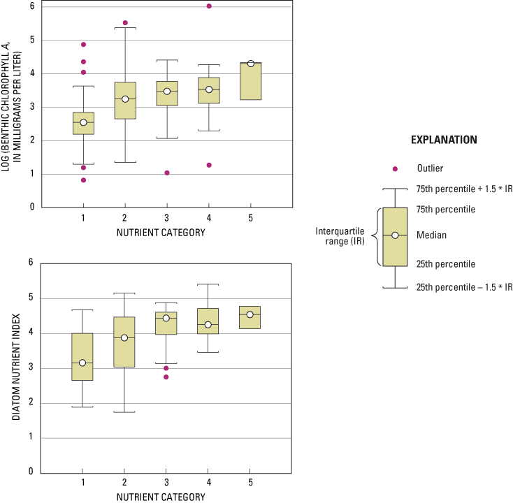
Figure 20. Benthic chlorophyll a concentrations and Diatom Nutrient Index values for five nutrient categories for the studied wadeable streams in Wisconsin.
The multimetric diatom index DBI was also tested as a means to define thresholds in the response of the diatom community to changes in nutrient concentrations. The DNI and DSI, however, provided more defined thresholds in the response of the diatom community to changes in nutrient concentrations, and, therefore, the DBI was not examined in further detail for this purpose.
Forward stepwise regressions were done with the water-quality (median values), environmental, and physical-habitat characteristics to determine which four characteristics best described the variance in BCHL concentrations and the diatom indices (table 14). Models with more than four variables did not significantly increase the amount of variance explained (accumulative R2 values). For BCHL, NO3-N concentration was the first variable incorporated in the model, whereas DP concentration was the first variable incorporated in the DNI and DBI models. The clay content of the soil was the first variable incorporated in the DSI model, followed by P concentration. The clay content of the soil indicates the potential for siltation and, therefore, was expected to be an important variable in the DSI model. With four variables, the models explained between 31 and 60 percent of the total variance in the indices; therefore, 40 to 70 percent of the variance was not explained by the characteristics examined in this study.
Table 14. Results of forward stepwise-regression analysis to explain the variance in benthic chlorophyll a concentrations and the three diatom indices in the studied wadeable streams in Wisconsin.
[R2, coefficient of determination for the one-, two-, three-, and four-variable models; all regressions were on log-transformed values of the dependant variable]
| Dependent variable | First variable | Second variable | Third variable | Fourth variable |
|---|---|---|---|---|
| Benthic chlorophyll a (BCHL) | Nitrite plus nitrate | Nonglacial deposits | Loam deposits | Runoff |
| Accumulative R2 | 0.32 | 0.37 | 0.40 | 0.43 |
| Diatom Nutrient Index (DNI) | Dissolved phosphorus | Wetland (forested) | Percentage of pools | Soil slope |
| Accumulative R2 | .25 | .31 | .33 | .34 |
| Diatom Siltation Index (DSI) | Clay content of soil | Total phosphorus | Nonglacial deposits | Grassland |
| Accumulative R2 | .42 | .49 | .59 | .60 |
| Diatom Biotic Index (DBI) | Dissolved phosphorus | Agriculture (row crops) | Wetland (forested) | Percentage of sand bottom |
| Accumulative R2 | .19 | .25 | .29 | .31 |
Partial RDA was used to determine the relative importance of nutrients, other water-quality characteristics (pH, specific conductance, water clarity, and flow), and environmental and physical-habitat characteristics (tables 2 and 10) in influencing the distribution of BCHL and the three diatom indices. In this analysis, individual monthly (July and August) and median values were included for each nutrient. A forward variable-selection procedure, which correlated the BCHL and the three diatom indices to the other factors, was used to select a subset of variables for each general type of characteristic. This procedure retained 7 nutrient variables, 5 other water-quality characteristics, and 11 environmental and physical-habitat characteristics. These final 23 characteristics explained 54 percent of the variance in BCHL and the diatom indices. Of the explained variance, 13 percent was explained by the nutrients alone, 4 percent by the other water-quality characteristics alone, 46 percent by the environmental and physical-habitat characteristics alone, and 37 percent by the interactions among all the characteristics (fig. 21). Therefore, nutrient concentrations by themselves explained only a small part (about 7 percent) of the total variance in BCHL and the diatom communities. About 46 percent of the total variance could not be explained with the characteristics examined in this study.
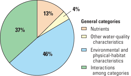
Figure 21. Percentage of explained variance in benthic chlorophyll a concentrations and diatom index values described by nutrients, other water-quality characteristics, environmental (anthropogenic/land-use, soil, and surficial-deposit characteristics) and physical-habitat characteristics, and interactions among categories (variance that can not be explained by a single category) for the studied wadeable streams in Wisconsin. [%, percentage of explained variance]
A reference BCHL concentration and reference values for the three diatom indices were determined by examining the concentrations and index values at only the sites having both P and N concentrations at or below their respective reference concentrations (35 Reference sites). The median BCHL concentration for the Reference sites was 331 mg/m2 (log (331) = 2.52; the 75th percentile was 673 mg/m2), which was significantly less than the median concentration measured at the High (nonreference) sites (3,020 mg/m2; log (3,020) = 3.48; fig. 22). The median DNI and DSI values for the Reference sites were 3.38 and 11.80, respectively (with 75th percentiles of 4.05 and 22.50, respectively), which were significantly less than the median values measured at the High sites (4.39 and 52.00, respectively). The median DBI value for the Reference sites was 47.5 (with a 25th percentile of 37.4; a lower percentile is given because a larger DBI represents a better diatom community), which was significantly greater than the median value measured at the High sites (39.9). If 75 percent of the minimally impacted sites (the Reference sites) have water-quality conditions or index values at least as good as the reference condition, then the reference concentration for BCHL is 673 mg/m2, and the reference index values for DNI, DSI, and DBI are 4.05, 22.5, and 37.4, respectively.
Comparing the median concentration and index values for the Reference sites with those for the Ref N and Ref P sites may provide an indication of whether P or N is more important in limiting the concentrations of BCHL and the degradation of the diatom community in streams with nutrient concentrations near reference conditions (fig. 22). For BCHL, it appears that N is the more important limiting nutrient because the median value for the Ref P sites was significantly higher than the median value for the Reference sites, and there was no statistical difference between median values for Reference sites and the Ref N sites. In other words, small additions of N (Ref P) had more of an effect on BCHL concentrations than small additions of P (Ref N). Small additions of N also may have had a small effect on DSI values, although the median values for the categories were not significantly different. Small additions of P and N had little effect on DNI and DBI values in streams with nutrient concentrations near reference conditions.
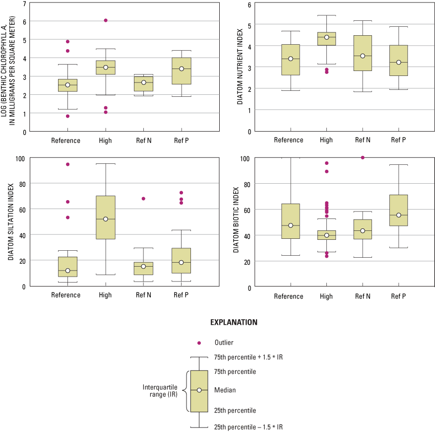
Figure 22. Benthic chlorophyll a concentrations, Diatom Nutrient Index, Diatom Siltation Index, and Diatom Biotic Index values in Reference sites, High (nonreference) sites, and sites with only reference total nitrogen (Ref N sites) or reference total phosphorus (Ref P sites) concentrations in the studied wadeable streams in Wisconsin. [log, logarithm to base 10 transformation]
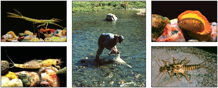 |
| Wisconsin Department of Natural Resources personnel collecting macroinvertebrate samples. Macroinvertebrate pictures provided by Stanley Szczytko (University of Wisconsin–Stevens Point). |
Six indices were used to describe the macroinvertebrate communities in the studied wadeable streams in Wisconsin (table 10). Hilsenhoff Biotic Index (HBI) values ranged from 0.8 to 9.4 (median = 4.7); the percentage of individuals that were either Ephemeroptera, Plecoptera, or Trichoptera (EPTN%) varied from 0.0 to 99.2 percent (median = 42.3 percent); the percentage of taxa that were Ephemeroptera, Plecoptera, or Trichoptera (EPTTX%) varied from 0.0 to 74.3 percent (median = 35.7 percent); the percentage of the individuals that were scrapers (SCRAP%) varied from 0.0 to 85.4 percent (median = 14.7 percent); the percentage of individuals that were shredders (SHRED%) varied from 0.0 to 24.7 percent (median = 0.0 percent), and the total numbers of taxa (TAXAN) varied from 4 to 67 (median = 29). In general, streams in the northern part of the State had macroinvertebrate communities that would normally be considered representative of better water quality, with lower HBI values, higher EPTN% and EPTTX% (fig. 23), and higher TAXAN than the streams in the southeastern part of the State. The SCRAP% and SHRED% did not exhibit strong regional patterns.
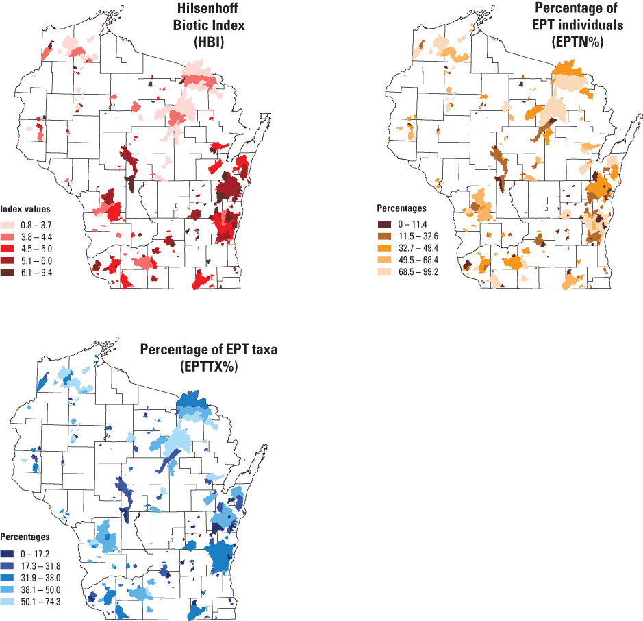
Figure 23. Distributions (quintiles) of macroinvertebrate Hilsenhoff Biotic Index (HBI) values, the percentages of individuals that were Ephemeroptera, Plecoptera, or Trichoptera (EPTN%), and the percentages of taxa that were Ephemeroptera, Plecoptera, or Trichoptera (EPTTX%) for the studied wadeable streams in Wisconsin.
Spearman rank correlation coefficients (rs values) between the six macroinvertebrate indices and median water-quality, environmental, and physical-habitat characteristics are given in table 15. All six indices were significantly correlated with at least two nutrient constituents. Of the six macroinvertebrate indices, HBI, EPTN%, and EPTTX% were most strongly correlated with the nutrients. HBI and EPTN% were significantly correlated with all of the nutrients except NO3-N. SCRAP% and TAXAN were negatively correlated with most nutrients, although many of the correlations were not statistically significant. Concentrations of P and N were positively correlated with HBI values and negatively correlated with EPTN%, EPTTX%, and TAXAN. Better macroinvertebrate indices (lower HBI values, higher EPT indices, and more taxa) occurred with lower nutrient concentrations. The SCRAP%, SHRED%, and TAXAN were less strongly correlated with most nutrient concentrations. Individual monthly nutrient concentrations were examined, but in all cases the monthly values explained less variance than the median values.
Table 15. Spearman rank correlation coefficients (rs) between macroinvertebrate-community indices and median water-quality, environmental (anthropogenic/land-use, basin, soil and surficial-deposit), and physical-habitat characteristics for the studied wadeable streams in Wisconsin.
[EPT, Ephemeroptera, Plecoptera, and Trichoptera; %, percent; all bold values were significant at p < 0.05, after being adjusted for the Bonferroni correction (Zar, 1999); see table 10 for definitions of abbreviations and units for each parameter]
| Characteristic | Hilsenhoff Biotic Index | Percentage of EPT individuals | Percentage of EPT taxa | Percentage of scrapers | Percentage of shredders | Number of taxa |
|---|---|---|---|---|---|---|
|
|
||||||
| Total phosphorus | 0.55 | -0.35 | -0.46 | -0.21 | 0.09 | -0.19 |
| Dissolved phosphorus | .50 | -.33 | -.43 | -.18 | .06 | -.18 |
| Total nitrogen | .37 | -.37 | -.39 | -.10 | -.06 | -.30 |
| Dissolved nitrite plus nitrate | .16 | -.24 | -.20 | .03 | -.21 | -.28 |
| Dissolved ammonia | .53 | -.39 | -.54 | -.21 | .12 | -.27 |
| Total Kjeldahl nitrogen | .54 | -.28 | -.44 | -.28 | .30 | -.10 |
| Suspended chlorophyll a | .42 | -.27 | -.33 | -.04 | .18 | .04 |
| Secchi tube depth | -.41 | .29 | .34 | .17 | -.11 | .23 |
| Urban | .16 | -.10 | -.03 | .00 | .06 | -.08 |
| Agriculture (row crops) | .45 | -.42 | -.45 | -.07 | -.04 | -.33 |
| Agriculture (all) | .43 | -.38 | -.42 | -.02 | -.06 | -.31 |
| Grassland | -.12 | -.02 | .08 | .18 | -.22 | -.15 |
| Wetland (open) | .17 | -.07 | -.11 | -.08 | .22 | .04 |
| Wetland (forested) | .04 | .11 | .04 | -.14 | .25 | .16 |
| Forest (all) | -.48 | .42 | .48 | .08 | .01 | .30 |
| Point-source loading of phosphorus | .14 | .05 | .05 | -.05 | .11 | .03 |
|
|
||||||
| Watershed area | -.13 | .24 | .17 | .05 | .09 | .23 |
| Air temperature | .36 | -.33 | -.33 | .01 | -.13 | -.30 |
| Precipitation | -.08 | -.03 | .11 | .25 | -.21 | -.09 |
| Runoff | -.32 | .27 | .26 | -.01 | .14 | .27 |
| Basin Slope | -.15 | .11 | .15 | .18 | -.26 | -.11 |
| Flow per unit area | -.30 | .22 | .27 | .17 | -.09 | .08 |
|
|
||||||
| Clay content | .24 | -.26 | -.24 | .07 | -.10 | -.31 |
| Erodibility | .29 | -.24 | -.28 | .07 | -.07 | -.21 |
| Organic-matter content | .05 | .02 | -.02 | -.21 | .31 | .13 |
| Permeability | -.20 | .20 | .22 | -.05 | .06 | .21 |
| Soil slope | -.39 | .28 | .42 | .23 | -.23 | .13 |
| Nonglacial deposits | -.10 | .05 | .09 | .18 | -.18 | -.03 |
| Clay deposits | .24 | -.19 | -.22 | -.16 | .10 | -.09 |
| Loam deposits | .04 | .09 | .04 | .03 | -.03 | .00 |
| Peat deposits | .09 | -.06 | -.13 | -.19 | .24 | .01 |
| Sand deposits | .02 | -.03 | -.01 | -.08 | .17 | .09 |
| Sand-and-gravel deposits | -.14 | .13 | .15 | -.07 | .07 | .11 |
| WIDTH | -0.20 | 0.35 | 0.25 | 0.09 | 0.11 | 0.31 |
| DEPTH | .00 | .13 | .04 | .00 | .12 | .10 |
| THALD | -.04 | .17 | .07 | .00 | .13 | .14 |
| GRAD | -.16 | .01 | .11 | .19 | -.26 | -.08 |
| POOL% | -.16 | .07 | .10 | .19 | -.17 | .03 |
| RIFF% | -.26 | .23 | .28 | .28 | -.28 | .01 |
| RUN% | .25 | -.19 | -.25 | -.28 | .26 | -.04 |
| SEDEP | .20 | -.20 | -.26 | -.27 | .15 | -.08 |
| SILT% | .41 | -.32 | -.43 | -.15 | .09 | -.11 |
| SAND% | -.18 | .06 | .16 | -.05 | -.03 | .12 |
| GRAV% | -.25 | .24 | .28 | .30 | -.22 | .04 |
| EMB% | .26 | -.26 | -.30 | -.31 | .15 | -.05 |
| ALGAE% | .25 | -.15 | -.23 | .04 | -.05 | -.13 |
| MACR% | .16 | -.08 | -.15 | -.14 | .13 | .15 |
| COVER% | .06 | .01 | -.07 | -.12 | .21 | .16 |
| SHADE% | -.09 | .04 | .05 | .00 | -.19 | -.15 |
| EROSION% | .02 | -.03 | .00 | .06 | -.21 | -.18 |
| BUFFER | .05 | -.07 | -.05 | -.04 | .08 | -.14 |
In general, HBI, EPTN%, and EPTTX% were also the indices most strongly correlated with SCHL, SD, and the anthropogenic/land-use characteristics, especially the percentages of total agriculture, row-crop agriculture, and forested areas. Better macroinvertebrate indices (lower HBIs and higher EPT indices) generally occurred in streams with lower SCHL and higher clarity, in areas with lower percentages of agriculture and higher percentages of forest. SCRAP%, SHRED%, and TAXAN were less strongly correlated with the anthropogenic/land-use characteristics. HBI, EPTN%, and EPTTX% were also more strongly correlated with the basin characteristics (air temperature, runoff, and flow per unit area) and the soil and surficial-deposit characteristics (clay content of the soil, erodibility, soil slope, and clay deposits) than were the other three macroinvertebrate indices. In general, better macroinvertebrate communities were found in areas with cooler air temperatures, higher runoff, soils with lower clay content, and higher soil slope. These areas with better macroinvertebrate indices are generally the mixed and mostly forested areas of Wisconsin (fig. 2A).
In general, the macroinvertebrate indices were only moderately correlated with the physical-habitat characteristics. The physical-habitat characteristics that were most strongly correlated with macroinvertebrate indices were the percentages of rocky-substrate embeddedness, percentages of riffles and runs, and percentages of silt and gravel sediment. Better macroinvertebrate communities were found in wider streams with lower percentages of runs, rocky-substrate embeddedness, and silt sediment, and higher percentages of riffles and gravel substrate. Many macroinvertebrate samples were collected in areas of the stream with physical-habitat characteristics that were substantially different from the average characteristics for the entire stream reach. Improved correlations between the physical-habitat characteristics and the macroinvertebrate indices would have probably occurred if the habitat characteristics were estimated for only the area near the macroinvertebrate-sampling location.
Responses in the three macroinvertebrate community indices most strongly correlated with nutrients (HBI, EPTN%, and EPTTX%) are shown in figures 24 and 25. In general, HBI values increased as nutrient concentrations increased, whereas EPTN% and EPTTX% values decreased or showed no clear trend with increases in nutrient concentrations. At low nutrient concentrations, the values of these macroinvertebrate measures ranged widely; however, at high nutrient concentrations, the values were generally poor (high HBI values and low EPT indices). The best relations were found between HBI values and P, DP, and TKN concentrations, and between both EPT indices and P, DP, and NH4-N concentrations. The other relations with nutrient concentrations ranged more widely; little relation was found between both EPT indices and N, TKN, and NO3-N concentrations. The lower bounds of HBI plots and the upper bounds of the EPT plots may provide an indication of how nutrients are capable of affecting the macroinvertebrate community. The variation below the HBI bounds and above the EPT bounds may indicate the effects caused by factors other than nutrients.
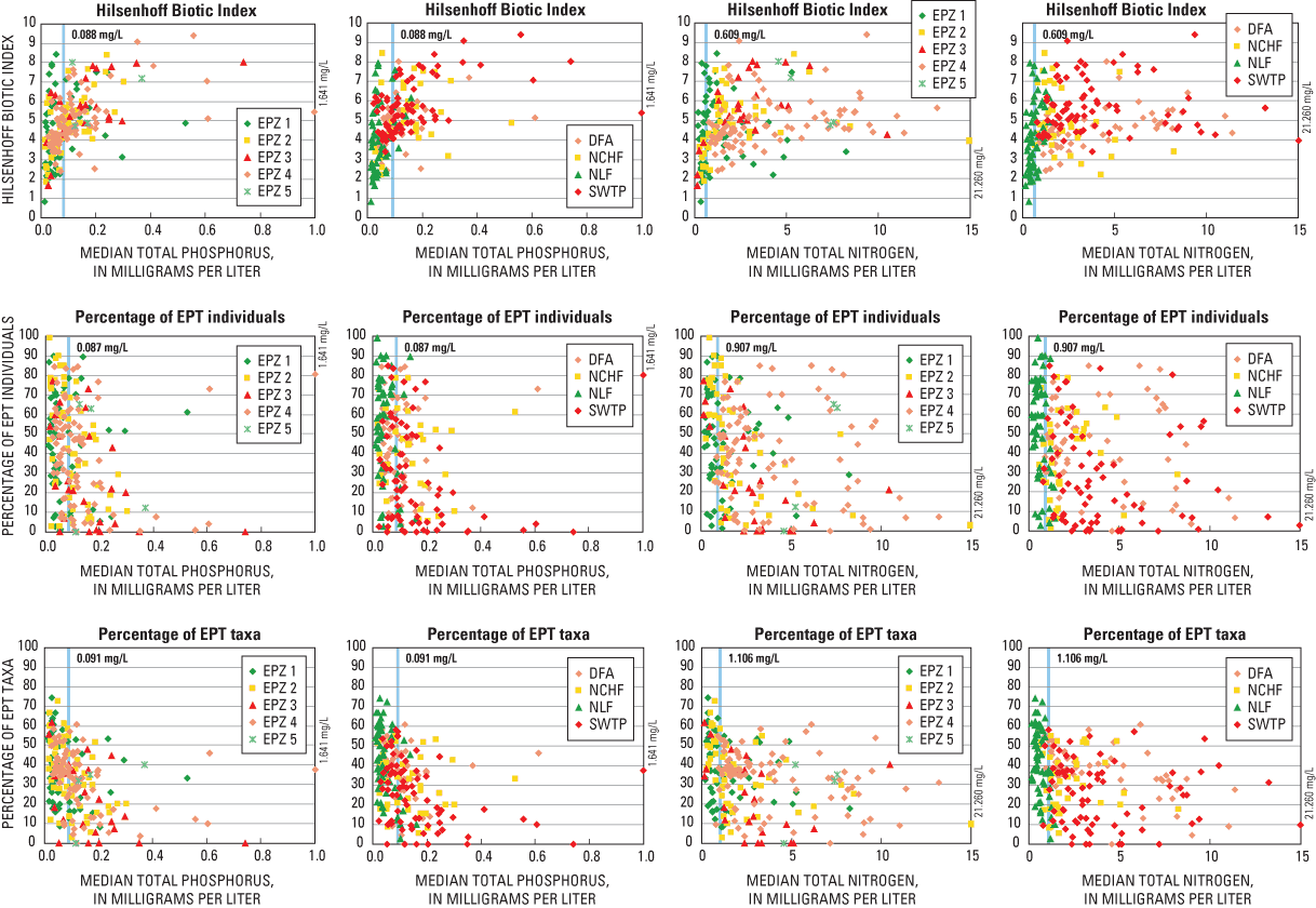
Figure 24. Hilsenhoff Biotic Index values, the percentages of individuals that were Ephemeroptera, Plecoptera, or Trichoptera, and the percentages of taxa that were Ephemeroptera, Plecoptera, or Trichoptera as a function of total phosphorus and total nitrogen concentration in the environmental phosphorus zones (EPZs) and level III ecoregions for the studied wadeable streams in Wisconsin. Computed thresholds in the response are identified by vertical lines. [DFA, Driftless Area; NCHF, North Central Hardwood Forests; NLF, Northern Lakes and Forests; and SWTP, Southeastern Wisconsin Till Plains]
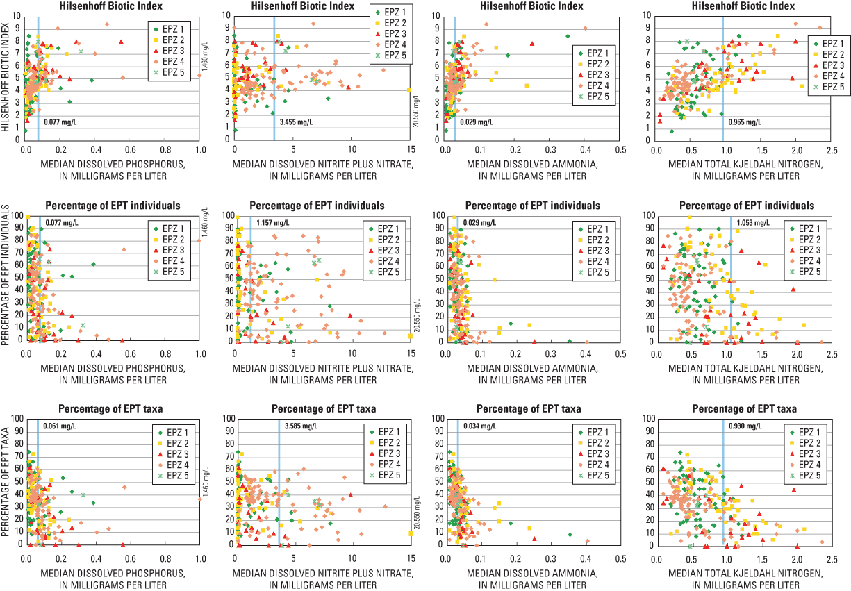
Figure 25. Hilsenhoff Biotic Index values, the percentages of individuals that were Ephemeroptera, Plecoptera, or Trichoptera, and the percentages of taxa that were Ephemeroptera, Plecoptera, or Trichoptera as a function of dissolved phosphorus, dissolved nitrite plus nitrate, dissolved ammonia, and total Kjeldahl nitrogen concentrations in the environmental phosphorus zones (EPZs) for the studied wadeable streams in Wisconsin. Computed thresholds in the response are identified by vertical lines.
Although nutrient concentrations were lower or higher in some EPZs and ecoregions (especially lower in EPZ 1 and the NLF ecoregion), macroinvertebrate indices responded similarly to changes in nutrient concentrations in all areas of the State (fig. 24). In all areas, there was a broad response at low nutrient concentrations and poor indices at high nutrient concentrations. Differences in the responses among areas could not be distinguished because of the range of the data and because the gradient in nutrient concentrations within some areas was small.
Regression-tree analyses were performed to define specific thresholds or breakpoints in the responses of the three macroinvertebrate community indices most strongly correlated with nutrients (table 16). The thresholds or breakpoints in the responses to changes in most nutrient concentrations were consistent among these three indices, although the data do not indicate well-defined thresholds. The thresholds in the responses to changes in total P concentrations were at about 0.09 mg/L, to changes in DP concentrations were at about 0.06–0.08 mg/L, to changes in total N concentrations were from 0.609 to 1.106 mg/L (the lowest threshold value occurred for HBI), to changes in NH4 -N concentrations were at about 0.03 mg/L, and to changes in TKN concentrations were at about 1.0 mg/L. The range in the thresholds to changes in NO3-N concentrations was broader (from 1.157 to 3.585 mg/L). In general, the macroinvertebrate indices ranged widely below the thresholds; however, macroinvertebrate indices were poor above the thresholds.
Table 16. Thresholds or breakpoints in the responses in macroinvertebrate indices to changes in nutrient concentrations for wadeable streams in Wisconsin.
[EPT, Ephemeroptera, Plecoptera, and Trichoptera; all concentrations are in milligrams per liter]
| Biological indices | Total phosphorus | Dissolved phosphorus | Total nitrogen | Dissolved nitrite plus nitrate | Dissolved ammonia | Total Kjeldahl nitrogen |
|---|---|---|---|---|---|---|
| Hilsenhoff Biotic Index (HBI) | 0.088 | 0.077 | 0.609 | 3.455 | 0.029 | 0.965 |
| Percentage of EPT individuals (EPTN%) | .087 | .077 | .970 | 1.157 | .029 | 1.053 |
| Percentage of EPT taxa (EPTTX%) | .091 | .061 | 1.106 | 3.585 | .034 | .938 |
Forward stepwise regressions were done with the median water-quality, environmental, and physical-habitat characteristics to determine which four characteristics best described the variance in the macroinvertebrate indices (table 17). Models with more than four variables did not significantly increase the amount of variance explained (accumulative R2 value). For most indices, either a nutrient or the percentage of forest/agriculture was the first variable incorporated in the models, except for the SCRAP% and SHRED% that were found to be weakly correlated with nutrient concentrations. Even with four variables, the models explained only 19 to 47 percent of the variance in the indices. The stepwise regressions explained the most variance in the same three macroinvertebrate indices (HBI, EPTN%, and EPTTX%) that were most related to the nutrients and environmental characteristics. The SHRED% model appears to have better predictability than the percent variance explained indicates because most of the values for SHRED% were 0.
Table 17. Results of forward stepwise-regression analyses to explain variance in macroinvertebrate indices for the studied wadeable streams in Wisconsin.
[EPT, Ephemeroptera, Plecoptera, and Trichoptera; R2, coefficient of determination for the one-, two-, three-, and four-variable models]
| Dependent variable | First variable | Second variable | Third variable | Fourth variable |
|---|---|---|---|---|
| Hilsenhoff Biotic Index (HBI) | Dissolved ammonia | Flow per unit area | Percentage of macrophyte cover | Total phosphorus |
| Accumulative R2 | 0.31 | 0.38 | 0.43 | 0.47 |
| Percentage of EPT individuals (EPTN%) | Forest (all) | Percentage of rocky- substrate embeddedness | Stream depth | Organic-matter content |
| Accumulative R2 | .19 | .28 | .32 | .35 |
| Percentage of EPT taxa (EPTTX%) | Dissolved ammonia | Agriculture (row crops) | Percentage of rocky-substrate embeddedness | Flow per unit area |
| Accumulative R2 | .26 | .35 | .42 | .45 |
| Percentage of scrapers (SCRAP%) | Precipitation | Sediment depth | Total phosphorus | Percentage of macrophyte cover |
| Accumulative R2 | .07 | .12 | .16 | .19 |
| Percentage of shredders (SHRED%) | Peat deposits | Kjeldahl nitrogen | Percentage of streambank with erosion | Percentage of silt |
| Accumulative R2 | .30 | .35 | .38 | .41 |
| Number of taxa (TAXAN) | Total nitrogen | Watershed area | Clay deposits | Buffer width |
| Accumulative R2 | .14 | .17 | .20 | .22 |
Partial RDA was used to determine the relative importance of the nutrients, other water-quality characteristics, and environmental and physical-habitat characteristics (tables 2 and 10) in affecting the distribution of the macro-invertebrate communities (the six macroinvertebrate-community indices). In this analysis, individual monthly (July and August) and median values were included for each nutrient. A forward variable-selection procedure, which correlated the macroinvertebrate indices with the other factors, was used to select a subset of variables for each general type of characteristic. This procedure retained 9 nutrient variables, 3 other water-quality characteristics, and 17 environmental and physical-habitat characteristics. These 29 characteristics explained 43 percent of the variance in the six macroinvertebrate-community indices. Of the explained variance, 22 percent was described by the nutrients alone, 5 percent by the other water-quality characteristics alone, 41 percent by the environmental and physical-habitat characteristics alone, and 32 percent by the interactions among all the characteristics (fig. 26). Therefore, nutrient concentrations by themselves explained only a small part (about 10 percent) of the total variance in the macroinvertebrate communities. About 57 percent of the total variance could not be explained by the characteristics examined in this study, and 14 percent of the total variance could not be separated into a single category of characteristics.
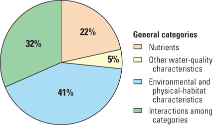
Figure 26. Percentages of explained variance in six macroinvertebrate index values described by nutrients, other water-quality characteristics, environmental (anthropogenic/land-use, soil, and surficial-deposit characteristics) and physical-habitat characteristics, and interactions among categories (variance that can not be explained by a single category) for the studied wadeable streams in Wisconsin. [%, percentage of explained variance]
Reference values for the three macroinvertebrate indices most related to nutrient concentrations (HBI, EPTN%, and EPTTX%) were determined by examining the index values at only the sites having both P and N concentrations at or below their respective reference concentrations. The median HBI value for the Reference sites was 3.1 (with a 75th-percentile value of 4.4), which was significantly less than the median value at the High (nonreference) sites (5.1; fig. 27). The median reference EPTN% and EPTTX% values were 60 and 50 percent, respectively (with 25th-percentile values of 51 and 38 percent, respectively; lower percentiles are given for these indices because larger values represent better macroinvertebrate communities), which were significantly more than the median values measured at the High sites (33 and 31 percent, respectively). If 75 percent of the minimally impacted sites (the Reference sites) have index values at least as good as the reference condition, then the reference index values for HBI, EPTN%, and EPTTX% are 4.4, 51 percent, and 38 percent, respectively.
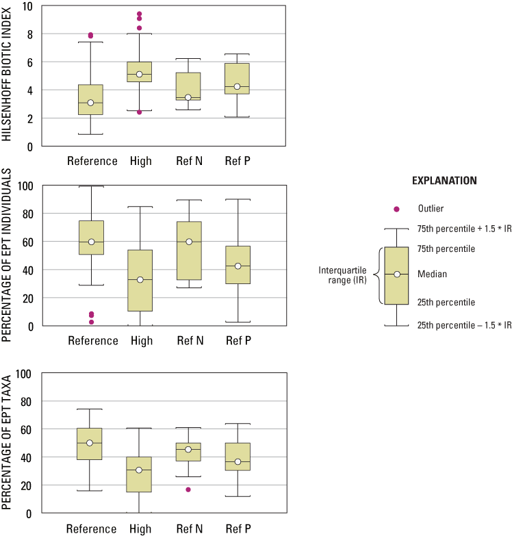
Figure 27. Hilsenhoff Biotic Index values, the percentages of individuals that were Ephemeroptera, Plecoptera, or Trichoptera, and the percentages of taxa that were Ephemeroptera, Plecoptera, or Trichoptera in Reference sites, High (nonreference) sites, and sites with only reference total nitrogen (Ref N sites) or reference total phosphorus (Ref P sites) concentrations in the studied wadeable streams in Wisconsin.
Comparing the median index values for the Reference sites with those for the Ref N and Ref P sites may provide an indication of whether P or N is more important in the degradation of the macroinvertebrate community in streams with nutrient concentrations near reference conditions (fig. 27). For all three indices, it appears that N is the more important limiting nutrient because the median values for the Ref P sites were significantly higher (HBI) or lower (EPTN% and EPTTX%) than the median values for the Reference sites. There were no differences between median values for Reference sites and the Ref N sites. Small additions of N (Ref P) had more of an effect on the macroinvertebrate communities than small additions of P (Ref N) for sites with nutrient concentrations near reference conditions.
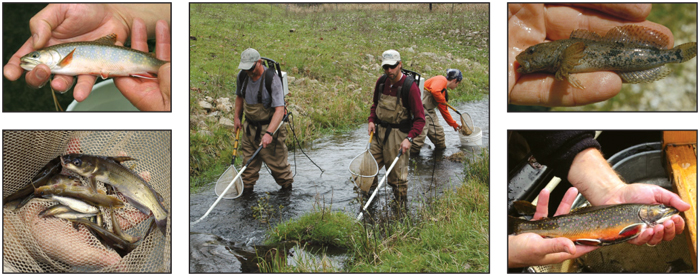 |
| Wisconsin Department of Natural Resources personnel collecting fish with electrofishing gear. Fish pictures provided by Michael Miller and John Lyons (Wisconsin Department of Natural Resources). |
The streams examined had a wide range in fish communities. Eight indices were used to describe the fish communities (table 10). Fish Index of Biotic Integrity (IBI) values ranged from 0.0 to 100.0 (median = 40.0). The percentages of fish considered carnivores (CARN%) and insectivores (INSECT%) ranged from 0.0 to 100.0 percent (median = 1.6 and 48.9 percent, respectively). The percentages of fish considered omnivores (OMNI%) ranged from 0.0 to 81.1 percent (median = 10.5 percent). The percentages of fish considered pollution intolerant (INTOL%) ranged from 0.0 to 97.9 percent (median = 3.3 percent), and the percentage of fish considered pollution tolerant (TOL%) ranged from 0.0 to 100.0 percent (median = 42.8 percent). The number of fish caught (FISHN) ranged from 7 to 2,147 fish (median = 130). The number of species of fish caught (FISHSPEC) ranged from 1 to 33 species (median = 11). Streams in the northern and central parts of the State generally had higher IBI, INTOL%, and CARN% than streams in other parts of the State (fig. 28). The INSECT%, OMNI%, TOL%, FISHN, and FISHSPEC did not exhibit strong regional patterns.
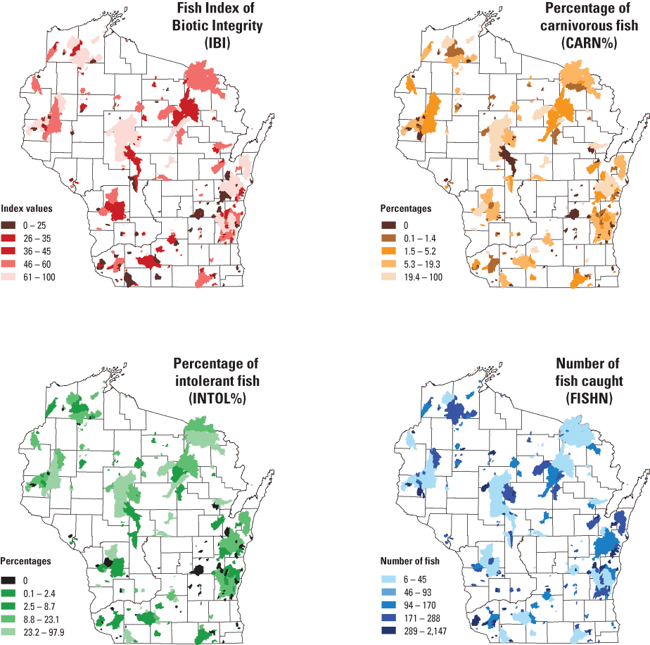
Figure 28. Distributions (quintiles) of fish Index of Biotic Integrity (IBI) values, the percentages of the fish that are carnivorous (CARN%), the percentages of fish considered pollution intolerant (INTOL%), and the number of fish caught (FISHN) for the studied wadeable streams in Wisconsin.
Spearman rank correlation coefficients between the eight fish indices and median water-quality, environmental, and physical-habitat characteristics are shown in table 18. All eight indices were significantly correlated with at least one nutrient constituent. IBI, CARN%, and INTOL% values were most strongly correlated with most nutrients. OMNI% and TOL% values were also significantly correlated with some nutrients, but less strongly correlated than these three indices. The other three indices (INSECT%, FISHSPEC, and FISHN) were significantly correlated with only NH4-N, TKN, or DP. In general, the fish indices indicative of better conditions (higher IBI, CARN%, INTOL% values) occurred with lower nutrient concentrations. Concentrations of NO3-N were significantly correlated with the smallest number of fish indices. Individual monthly nutrient concentrations were also examined, but in all cases explained less variance than the median values.
Table 18. Spearman rank correlation coefficients (rs) between fish-community indices and median water-quality, environmental (anthropogenic/land-use, basin, soil, and surficial-deposit), and physical-habitat characteristics for the studied wadeable streams in Wisconsin.
[all bold values were significant at p < 0.05, after being adjusted for the Bonferroni correction (Zar, 1999); see table 10 for definitions of abbreviations and units for each parameter]
| Characteristic | Fish Index of Biotic Integrity | Percentage of carnivores | Percentage of insectivores | Percentage of omnivores | Percentage of intolerant species | Percentage of tolerant species | Number of fish species | Number of fish |
|---|---|---|---|---|---|---|---|---|
|
|
||||||||
| Total phosphorus | -0.33 | -0.42 | 0.13 | 0.23 | -0.36 | 0.24 | 0.12 | 0.18 |
| Dissolved phosphorus | -.29 | -.41 | .09 | .21 | -.36 | .22 | .12 | .23 |
| Total nitrogen | -.31 | -.29 | .09 | .26 | -.31 | .08 | -.07 | .14 |
| Dissolved nitrate plus nitrite | -.20 | -.14 | -.04 | .27 | -.17 | -.04 | -.10 | .12 |
| Dissolved ammonia | -.27 | -.46 | .23 | .16 | -.39 | .29 | .04 | .16 |
| Total Kjeldahl nitrogen | -.25 | -.43 | .29 | .11 | -.40 | .36 | .24 | .08 |
| Suspended chlorophyll a | -.04 | -.28 | .18 | .26 | -.20 | .03 | .33 | .15 |
| Secchi tube depth | .32 | .36 | -.11 | -.29 | .38 | -.17 | -.05 | .01 |
| Urban | .03 | .10 | .13 | .15 | .04 | -.05 | .12 | -.17 |
| Agriculture (row crops) | -.25 | -.37 | .13 | .26 | -.41 | .13 | .03 | .22 |
| Agriculture (all) | -.26 | -.36 | .09 | .29 | -.37 | .09 | .04 | .27 |
| Grassland | .06 | .00 | -.02 | .07 | .09 | -.03 | -.07 | -.01 |
| Wetland (open) | .14 | -.09 | .30 | .05 | .00 | .06 | .34 | -.08 |
| Wetland (forested) | .13 | .04 | .19 | -.22 | .05 | .12 | .16 | -.21 |
| Forest (all) | .28 | .39 | -.11 | -.31 | .40 | -.13 | -.05 | -.24 |
| Point-source loading of phosphorus | .09 | .16 | .05 | .21 | .11 | -.11 | .30 | -.23 |
| Watershed area | .26 | .34 | .08 | .24 | .25 | -.25 | .47 | -.20 |
| Air temperature | -.32 | -.30 | .04 | .35 | -.42 | .15 | -.05 | .25 |
| Precipitation | -.15 | -.06 | -.17 | .20 | -.12 | .02 | -.05 | .14 |
| Runoff | .26 | .26 | -.11 | -.28 | .37 | -.16 | .04 | -.17 |
| Basin slope | -.12 | .05 | -.22 | .10 | -.01 | -.04 | -.18 | .12 |
| Unit area flow | .07 | .08 | -.06 | -.09 | .20 | .03 | -.02 | .02 |
| Clay content | -.27 | -.25 | -.02 | .26 | -.33 | .09 | -.05 | .23 |
| Erodibility | -.28 | -.35 | -.05 | .28 | -.35 | .10 | .07 | .38 |
| Organic-matter content | .16 | .12 | .18 | -.18 | .04 | .05 | .10 | -.25 |
| Permeability | .26 | .27 | .11 | -.20 | .26 | -.10 | .01 | -.29 |
| Soil slope | .05 | .30 | -.22 | -.02 | .24 | -.16 | -.16 | -.03 |
| Nonglacial deposits | -.13 | .04 | -.16 | .20 | .00 | -.12 | -.07 | .13 |
| Clay deposits | -.02 | .01 | .12 | .05 | -.14 | -.02 | .09 | -.07 |
| Loam deposits | .09 | .02 | .12 | -.14 | .18 | -.07 | .13 | -.18 |
| Peat deposits | .05 | .03 | .18 | .00 | .06 | -.11 | .15 | -.12 |
| Sand deposits | .12 | -.04 | .05 | -.14 | .04 | .02 | .03 | -.02 |
| Sand-and-gravel deposits | .21 | .19 | .09 | -.03 | .11 | -.01 | .11 | -.26 |
|
|
||||||||
| WIDTH | 0.31 | 0.35 | 0.02 | 0.17 | 0.31 | -0.28 | 0.54 | -0.17 |
| DEPTH | .04 | .15 | .12 | .32 | .13 | -.10 | .25 | -.21 |
| THALD | .08 | .22 | .12 | .29 | .18 | -.15 | .26 | -.24 |
| GRAD | -.11 | -.19 | -.18 | -.10 | -.15 | .04 | -.16 | .36 |
| POOL% | -.03 | -.01 | -.20 | .03 | -.05 | .01 | .07 | .29 |
| RIFF% | .14 | .00 | -.17 | -.07 | -.01 | -.11 | .21 | .26 |
| RUN% | -.03 | .03 | .24 | .01 | .07 | .08 | -.13 | -.31 |
| SEDEP | -.13 | .03 | .12 | -.01 | .01 | .07 | -.30 | -.29 |
| SILT% | -.40 | -.32 | .09 | .18 | -.39 | .25 | -.25 | .20 |
| SAND% | .15 | .27 | -.05 | -.15 | .27 | -.05 | -.11 | -.31 |
| GRAV% | .15 | -.01 | -.18 | .03 | .03 | -.03 | .39 | .23 |
| EMB% | -.19 | -.01 | .11 | -.04 | -.03 | .11 | -.40 | -.23 |
| ALGAE% | -.11 | -.25 | .00 | .18 | -.22 | .05 | .14 | .33 |
| MACR% | -.07 | .02 | .08 | -.04 | -.03 | -.02 | -.10 | .13 |
| COVER% | .11 | .08 | .12 | .05 | .07 | .01 | .02 | -.10 |
| SHADE% | .01 | .03 | -.13 | -.08 | .02 | .03 | -.06 | -.10 |
| EROSION% | -.11 | -.06 | -.16 | .12 | -.04 | .03 | .10 | .01 |
| BUFFER | .07 | .07 | .12 | -.08 | .03 | -.06 | .07 | -.23 |
In general, IBI, CARN%, INTOL%, OMNI%, and FISHAB were the indices most strongly correlated with SCHL, SD, and the anthropogenic/land-use characteristics than were the other indices. These fish indices were most strongly correlated with the percentage of total agriculture, row-crop agriculture, and forested areas. Better fish indices (high IBI, CARN%, and INTOL% values) occurred with lower percentages of agriculture and higher percentages of forest. INSECT%, TOL%, and FISHSPEC were less strongly correlated with most of the anthropogenic/land-use characteristics than were IBI, CARN%, and INTOL%. IBI, CARN%, OMNI%, and INTOL% were more strongly correlated with several basin characteristics (watershed area, air temperature, and runoff) and soil characteristics (clay content, erodibility, permeability, and soil slope) than were INSECT%, TOL%, and FISHSPEC. In general, streams with better fish indices have larger drainage areas, cooler air temperatures, higher runoff, and soils with lower clay content, lower erodibility, and higher permeability. These areas with better fish indices, again, are generally the mixed and mostly forested areas of Wisconsin (fig. 2A).
In general, most fish indices were significantly correlated with only a few physical-habitat characteristics except for FISHSPEC and FISHN, which were significantly correlated with many of the characteristics. The physical-habitat characteristics most strongly correlated with fish indices were stream width and the percentage of silt in the bottom sediments. Better fish communities occurred in wider streams with lower percentages of silt in the sediments. More fish and more fish species were caught in streams with higher percentages of pools and riffles, gravel bottoms having less accumulated sediment (shallower sediment depths), lower percentages of rocky-substrate embeddedness, and a higher percentage of algal cover. More fish but fewer fish species were caught in narrower, shallower streams with steeper gradients.
Responses of the three fish-community indices most strongly correlated with nutrient concentrations (IBI, CARN%, and INTOL%) are shown in figures 29 and 30. In general, IBI, CARN%, and INTOL% values decrease with increases in P and DP concentrations; however, no consistent pattern is apparent in the relations of these indices to changes in concentrations of the N constituents, except for NH4-N. At low total P, DP, and NH4-N concentrations, the values of these fish indices ranged widely; however, at high nutrient concentrations, the values were generally indicative of poor water quality (low values). The upper bounds of the IBI, CARN%, and INTOL% plots may provide an indication of how P, DP, and NH4-N are capable of affecting the fish community. As was true for the other biotic indices, the variability below these bounds may be indicative of the effects of factors other than nutrients.
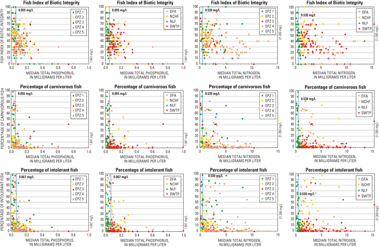
Figure 29. Fish Index of Biotic Integrity values, the percentages of fish considered pollution intolerant, and the percentages of the fish that are carnivorous as a function of total phosphorus and total nitrogen concentration in the environmental phosphorus zones (EPZs) and level III ecoregions for the studied wadeable streams in Wisconsin. Computed thresholds in the response are identified by vertical lines. [DFA, Driftless Area; NCHF, North Central Hardwood Forests; NLF, Northern Lakes and Forests; and SWTP, Southeastern Wisconsin Till Plains]
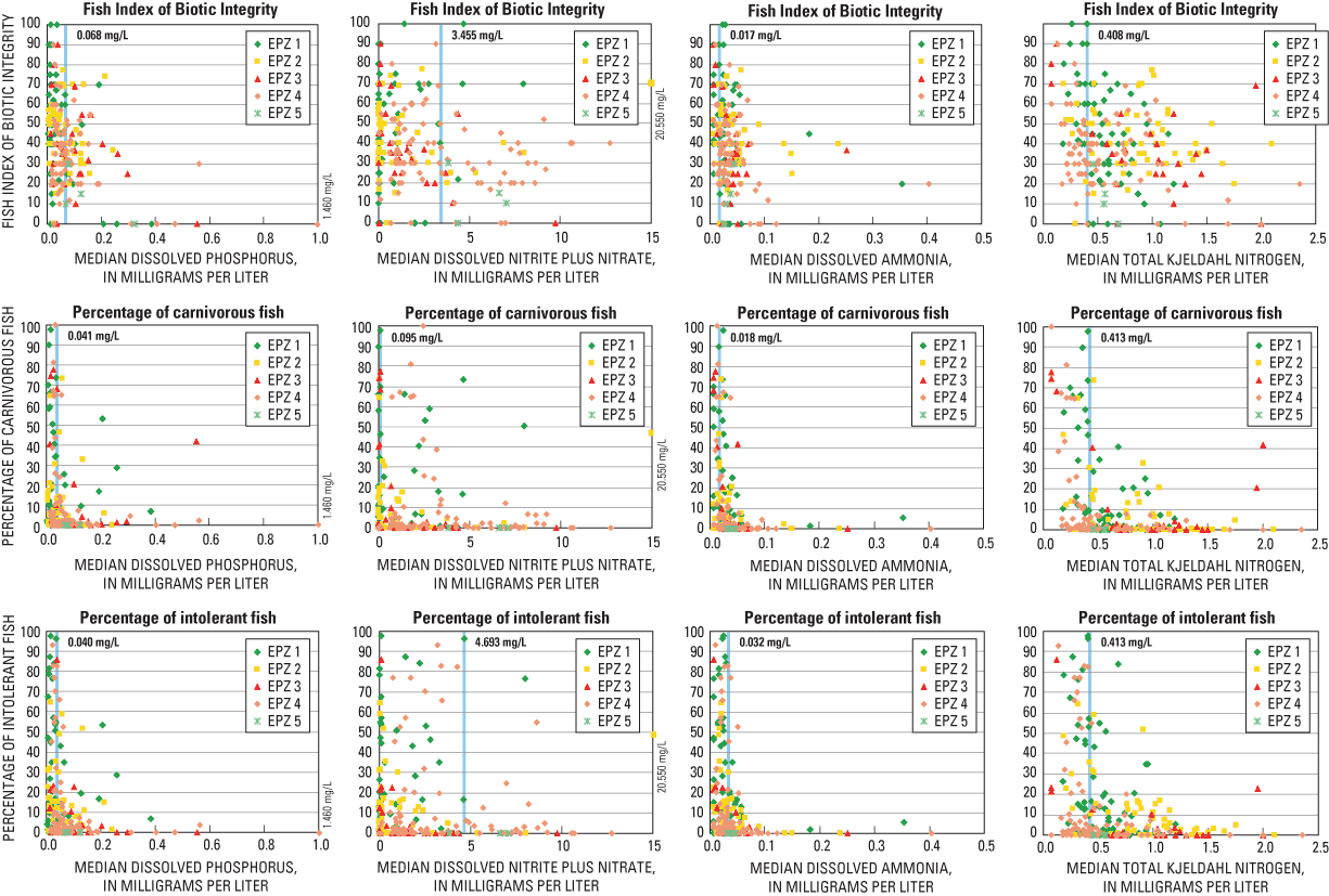
Figure 30. Fish Index of Biotic Integrity values, the percentages of fish considered pollution intolerant, and the percentages of the fish that are carnivorous as a function of dissolved phosphorus, dissolved nitrite plus nitrate, dissolved ammonia, and total Kjeldahl nitrogen concentrations in the environmental phosphorus zones (EPZs) for the studied wadeable streams in Wisconsin. Computed thresholds in the response are identified by vertical lines.
Relations between selected fish indices and nutrient concentrations appear to be similar in the various EPZs and ecoregions (fig. 29). In all areas, there was a broad response at low nutrient concentrations and lower indices (generally indicative of poor water quality) at high nutrient (P, DP, and NH4-N) concentrations. As for the other biotic indices, no significant differences in the responses were found among areas because of the range in the data, and because the gradient in nutrient concentrations within some areas was small.
Regression-tree analyses were done to define specific thresholds or breakpoints in the responses of the three fish-community indices that were most strongly correlated with the nutrient concentrations (table 19). The thresholds or breakpoints in the responses to changes in nutrient concentrations were consistent among these three indices. The thresholds in the responses to changes in P concentrations were about 0.06 mg/L, to changes in DP concentrations were from about 0.04 to 0.07 mg/L, and to changes in NH4-N concentrations thresholds were about 0.02–0.03 mg/L. In general, below these thresholds the fish indices ranged widely, but were consistently poor above these thresholds. The regression-tree analyses defined specific thresholds for N, TKN, and NO3-N; however, the data in figures 29 and 30 do not indicate any change in the indices with changes in the concentrations of these constituents.
Table 19. Thresholds or breakpoints in the responses in fish indices to changes in nutrient concentrations for wadeable streams in Wisconsin.
[all concentrations are in milligrams per liter]
| Biological Indices | Total Phosphorus | Dissolved phosphorus | Total nitrogen | Dissolved nitrite plus nitrate | Dissolved ammonia | Total Kjeldahl nitrogen |
|---|---|---|---|---|---|---|
| Fish Index of Biotic Integrity (IBI) | 0.055 | 0.068 | 0.539 | 3.455 | 0.017 | 0.408 |
| Percentage of carnivorous fish (CARN%) | .055 | .041 | .539 | .095 | .018 | .413 |
| Percentage of intolerant fish (INTOL%) | .067 | .040 | .539 | 4.693 | .032 | .413 |
Forward stepwise regressions were done with the median water-quality, environmental, and physical-habitat characteristics to determine which four characteristics best described the variance in the fish indices (table 20). Models with more than four variables did not significantly increase the amount of variance explained. For most indices, either P or TKN concentration was the first variable incorporated in these models. If TKN concentrations were not included in these models, then P concentrations became the first variable in the models. Other important variables included the width and depth of the streams and characteristics describing the substrate of the stream bottom. As was true for many other biotic-index models, even with four variables included, the relations only explained a small part of the total variance in these indices (in this case, from 22 to 42 percent). The model that explained the most variance was for FISHSPEC, which had watershed area and bottom substrate as the first two variables incorporated in the model.
Table 20. Results of forward stepwise-regression analyses to explain variance in fish indices for the studied wadeable streams in Wisconsin.
[R2, coefficient of determination for the one-, two-, three-, and four-variable models; log, logarithm to base 10 transformation]
| Dependent variable | First variable | Second variable | Third variable | Fourth variable |
|---|---|---|---|---|
| Fish Index of Biotic Integrity (IBI) | Total phosphorus | Stream width | Percentage of silt | Wetland (forested) |
| Accumulative R2 | 0.14 | 0.21 | 0.25 | 0.27 |
| Percentage of carnivorous fish (CARN%) | Kjeldahl nitrogen | Nonglacial deposits | Buffer width | Runoff |
| Accumulative R2 | .23 | .29 | .31 | .32 |
| Percentage of insectivorous fish (INSECT%) | Kjeldahl nitrogen | Percentage of pools | Percentage of gravel | Stream width |
| Accumulative R2 | .10 | .16 | .18 | .22 |
| Percentage of omnivorous fish (OMNI%) | Air temperature | Stream depth | Buffer width | Point-source loading of phosphorus |
| Accumulative R2 | .15 | .22 | .27 | .29 |
| Percentage of tolerant fish (TOL%) | Kjeldahl nitrogen | Stream width | Flow per unit area | Soil slope |
| Accumulative R2 | .15 | .21 | .23 | .24 |
| Percentage of intolerant fish (INTOL%) | Kjeldahl nitrogen | Stream width | Flow per unit area | Soil slope |
| Accumulative R2 | .15 | .26 | .27 | .29 |
| Number of fish species (FISHSPEC) | Watershed area | Percentage of gravel | Kjeldahl nitrogen | Buffer width |
| Accumulative R2 | .27 | .35 | .41 | .42 |
| Number of fish caught - log (FISHN) | Erodibility | Thalweg depth | Percentage of stream shaded | Percentage of gravel |
| Accumulative R2 | .15 | .23 | .26 | .30 |
Partial RDA was used to determine the relative importance of the nutrients, other water-quality characteristics, and environmental and physical-habitat characteristics (tables 2 and 10) in affecting the distribution of the fish communities (the eight fish indices). In this analysis, individual monthly (July and August) and median values were included for each nutrient constituent. A forward variable-selection procedure, which correlated fish indices with the other factors, was used to select a subset of variables for each general type of characteristic. This procedure retained 8 nutrient variables, 3 other water-quality characteristics, and 20 environmental and physical-habitat characteristics. These 31 characteristics explained 44 percent of the variance in the 8 fish-community indices. Of the explained variance, 15 percent was described by the nutrients alone, 3 percent by the other water-quality characteristics alone, 46 percent by the environmental and physical-habitat characteristics alone, and 36 percent by the interactions among all characteristics (fig. 31). About 56 percent of the total variance could not be explained with the characteristics examined in this study, and 16 percent of the total variance could not be separated into a single category of characteristics.
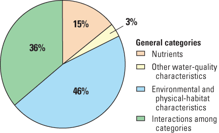
Figure 31. Percentages of explained variance in eight fish index values described by nutrients, other water-quality characteristics, environmental (anthropogenic/land-use, soil, and surficial-deposit characteristics) and physical-habitat characteristics, and interactions among categories (variance that can not be explained by a single category) for the studied wadeable streams in Wisconsin. [%, percentage of explained variance]
Reference values for the three fish indices that were most related to nutrient concentrations (IBI, CARN%, and INTOL%) were determined by examining the index values at only the sites having both P and N concentrations at or below their respective reference concentrations. The median IBI value for the Reference sites was 50 (with a 25th percentile of 40), the median reference CARN% value was 9.9 percent (with a 25th percentile of 1.5 percent), and the median reference INTOL% value was 14.7 percent (with a 25th percentile of 2.0 percent). Lower percentiles are given because larger values represent better fish communities. These median values were significantly higher than the median values measured at the High sites (35, 0.3 percent, and 2.0 percent respectively; fig. 32). If 75 percent of the minimally impacted sites (the Reference sites) had index values at least as good as the reference condition, then the reference index values for IBI, CARN%, and INTOL% are 40, 9.9 percent, and 2.0 percent, respectively.
Figure 32. Fish Index of Biotic Integrity values, the percentages of the fish that are carnivorous, and the percentages of fish that are considered pollution intolerant in Reference sites, High (nonreference) sites, and sites with only reference total nitrogen (Ref N sites) or reference total phosphorus (Ref P sites) concentrations in the studied wadeable streams in Wisconsin.
Comparing the median index values for the Reference sites with those for the Ref N and Ref P sites may provide an indication of whether P or N is more important in the degradation of the fish communities in streams with nutrient concentrations near reference conditions (fig. 32). For all three indices, there was no difference between median values for Reference sites and median values of the Ref N sites and Ref P sites. Therefore, small additions of P or N appear to have little effect on the fish communities in streams with nutrient concentrations near reference conditions.
One goal of this study was to estimate nutrient concentrations in streams from the biotic data. Most of the biotic indices, however, had a wedge-shaped response to increases in nutrient concentrations. In other words, there was a broad response in almost all index values at low nutrient concentrations; however, at high nutrient concentrations, the indices had a narrow range of values normally indicative of poor conditions. This wedge-shaped response of the biotic indices to increases in nutrient concentrations is common in describing relations between biotic indices and human disturbance levels, such as the percentage of urban land use in an area (Wang and others, 2001; 2003). The wedge-shaped response implies that at low nutrient concentrations, factors other than nutrients are predominant factors limiting the health of biotic communities, whereas at high nutrient concentrations, nutrients may be the predominant factors affecting biotic communities (Cade and others, 1999). Although these relations between nutrient concentrations and biotic indices have rarely been reported for wadeable streams in the literature, relations similar to those found in this study have been reported between P concentrations and percentages of gastropods and predator macroinvertebrates in P-addition experiments in Everglades sloughs (King and Richardson, 2004).
The wedge-shaped distribution makes predictions of low nutrient concentrations difficult with any single index. A combination of various biotic indices was used to assess whether this wedge-shaped response could be eliminated or at least reduced. To develop multiparameter indices to estimate P and N concentrations in wadeable streams, each of the indices found to be strongly related to changes in the nutrient concentrations was input into forward stepwise-regression analyses. Eleven biotic indices were included in this analysis: two describing chlorophyll a concentrations in the streams (log SCHL and log BCHL), three describing the periphytic-diatom community (DNI, DPTI, and DSI), three describing the macroinvertebrate community (HBI, EPTN%, and EPTTX%), and three describing the fish community (IBI, INTOL%, and CARN%).
The four-parameter model to estimate P concentrations in wadeable streams included indices describing the diatom community (DSI and DNI), suspended chlorophyll a (SCHL), and the fish community (IBI), and explained 54 percent of the variance in P concentrations (table 21). Models with more than four variables did not significantly increase the amount of variance explained (accumulative R2 value). Measured and estimated log P concentrations are shown in figure 33A. This multiparameter model estimated high and low P concentrations equally well.
Table 21. Results of forward stepwise-regression analyses to explain variance in total phosphorus and total nitrogen concentrations with biotic indices in the studied wadeable streams in Wisconsin.
[log, logarithm to base 10 transformation; rs, Spearman correlation coefficient; R2, coefficient of determination for the one-, two-, three-, and four-variable models; SCHL, suspended chlorophyll a concentration; na, not applicable; all regressions were on log-transformed concentrations; see table 10 for definitions of abbreviations and units for each parameter]
| Statistical parameter | Constant | First variable | Second variable | Third variable | Fourth variable |
|---|---|---|---|---|---|
|
|
|||||
| Diatom DSI | Log (SCHL) | Diatom DNI | Fish IBI | ||
| Coefficient in equation | -1.797 | 0.005 | 0.300 | 0.140 | -0.004 |
| rs | na | .60 | .44 | .47 | -.33 |
| Accumulative R2 | na | .32 | .41 | .48 | .54 |
|
|
|||||
| Log (BCHL) | EPTTX% | Fish IBI | Diatom DNI | ||
| Coefficient in equation | -0.373 | .200 | -.007 | -.005 | .108 |
| rs | na | .49 | -.39 | -.31 | .36 |
| Accumulative R2 | na | .23 | .33 | .37 | .41 |
Figure 33. Measured and estimated A, total phosphorus and B, total nitrogen concentrations (logarithm to base 10 transformation) for the four-parameter regression models, C , measured phosphorus concentrations as a function of Biotic Index of total Phosphorus (BIP) values, and D, measured nitrogen concentrations as a function of Biotic Index of total Nitrogen (BIN) values, with the regression equations and coefficients of determination (R2) for the studied wadeable streams in Wisconsin.
The four-parameter model to estimate N concentrations included indices describing benthic chlorophyll a (BCHL), the diatom community (DNI), the macroinvertebrate community (EPTTX%), and the fish community (IBI). This model explained 41 percent of the variance in N concentrations (table 21). Models with more than four variables did not significantly increase the amount of variance explained. Measured and estimated log N concentrations are shown in figure 33B. This multiparameter model estimated high and low N concentrations equally well, but did not estimate N concentrations as well as the P model estimated P concentrations.
The regression equations described in table 21 were then used to develop multiparameter biotic indices to estimate P and N concentrations in wadeable streams. The indices were developed to provide values ranging from 1 to 10, with 1 representing the lowest P and N concentrations and 10 representing the highest concentrations.
The Biotic Index of total P (BIP) is computed as:
| BIP = 4.0(-1.797 + 0.005DSI + 0.300Log SCHL + 0.140DNI – 0.004IBI) + 9.0, | (12) |
The Biotic Index of total N (BIN) is computed as:
BIN = 5.0(-0.373 + 0.200LogBCHL – 0.007EPTTX% – 0.005IBI + 0.108DNI) + 4.5, |
(13) |
The BIP and BIN values are plotted against their respective measured P and N concentrations in figures 33C and D. Both BIP and BIN estimate median P and N concentrations equally well over the range of concentrations measured in this study. The BIP predicted P concentrations better than the BIN predicted N concentrations (54 percent of the variance in P concentrations compared to 41 percent of the variance in N concentrations). The difference in the predictability of these indices was consistent with most of the biotic indices being more strongly correlated with P concentrations than with N concentrations. This difference in predictability suggests that P concentrations are more important than N concentrations in affecting the biotic communities over the range in nutrient concentrations measured in this study.
Excessive nutrient loss from watersheds is frequently associated with degraded water quality in streams. To reduce this loss from agricultural areas, performance standards and regulations for croplands and livestock operations are being proposed by various States. In addition, the USEPA is establishing regionally based nutrient criteria that can be refined by each State to determine whether actions are needed to improve a stream's water quality. More confidence in the environmental benefits of the proposed standards and nutrient criteria are possible with a better understanding of the biotic responses to a range of nutrient concentrations in different environmental settings.
To provide the information needed to guide the development of regionally based nutrient criteria for Wisconsin streams, the USGS and WDNR collected water-quality and biotic data in 240 wadeable streams throughout Wisconsin to: 1) describe how nutrient concentrations and biotic-community structure vary throughout the State; 2) determine which environmental characteristics are most strongly related to the distribution of nutrient concentrations; 3) determine reference water-quality and biotic conditions for different areas of the State; 4) determine how the biotic community of streams in different areas of the State respond to changes in nutrient concentrations; 5) determine the best regionalization scheme to describe the patterns in reference conditions and the responses in water quality and the biotic community; and 6) develop new indices to estimate nutrient concentrations in streams from a combination of biotic indices.
Two regionalization schemes were proposed for defining nutrient criteria for Wisconsin's wadeable streams: level III ecoregions and environmental phosphorus zones (EPZs). On the basis of the results of this study, the EPZ regionalization scheme was better than the level III ecoregion scheme at defining differences in reference water quality and differences in the responses in water quality to changes in land use for constituents that varied regionally. For some water-quality characteristics, however, the results indicated that little consistent variability was present and no regionalization was warranted. For total nitrogen (N) concentrations, suspended chlorophyll a (SCHL) and Secchi tube depth (SD), the regional variabilities in reference conditions and in the water-quality responses are best described by subdividing wadeable streams into two categories: streams in areas with high clay-content soils (EPZ 3) and streams throughout the rest of the State (fig. 34). The regional variability in the response in total phosphorus (P) concentrations to changes in land use was also best described by subdividing the streams into these two categories; however, little consistent variability was found in reference P concentrations in streams throughout the State.
Figure 34. Proposed regionalization scheme for defining nutrient criteria for wadeable streams in Wisconsin.
Despite variation in nutrient concentrations among EPZs and level III ecoregions (especially lower nutrient concentrations in the northern part of the State), the responses of all of the biotic indices to changes in nutrient concentrations were similar throughout the State. In all areas, there was a broad response in the indices at low nutrient concentrations and a narrower range in values, indicative of poor water quality, at high nutrient concentrations. No regional differences were found in the biotic responses among areas; therefore, there is no reason to subdivide the streams based on the biotic response to changes in nutrient concentrations.
Results of this study indicate that reference P concentrations for wadeable streams are similar throughout the State: 0.03–0.04 mg/L with an upper 95-percent confidence limit of 0.04–0.06 mg/L (table 22). These values are higher than those estimated by Robertson and others (2006), who estimated that reference P concentrations for Wisconsin streams and larger rivers were between 0.012 and 0.023 mg/L. Values from this study are similar to those defined by the USEPA for nutrient ecoregion 7, but higher than those defined for nutrient ecoregion 8. The USEPA defined reference P concentrations for the DFA and SWTP ecoregions at 0.070 and 0.080 mg/L, respectively, which are higher than those estimated in this study. The higher values defined for the DFA and SWTP ecoregions were probably because most of the watersheds of streams in those areas are dominated by agriculture, and more than 25 percent of the streams are affected by anthropogenic factors.
Table 22. Reference conditions for water quality, chlorophyll a, diatoms, macroinvertebrates, and fish indices for wadeable streams in Wisconsin.
[EPT, Ephemeroptera, Plecoptera, and Trichoptera; %, percent; mg/L, milligram per liter; µg/L, microgram per liter; cm, centimeter; >, greater than; mg/m 2 , milligram per square meter]
| Median reference | Upper 95-percent confidence limits | |
|---|---|---|
| Total phosphorus (P) (mg/L) | ||
| Entire State | 0.03–0.04 | 0.04–0.06 |
| Total nitrogen (N) (mg/L) | ||
| High-clay content areas (EPZ 3) | 0.4 | 0.6 |
| Rest of State | 0.6–0.7 | 0.7–1.0 |
| Suspended chlorophyll a (SCHL)(µg/L) | ||
| High-clay content areas (EPZ 3) | 1.0 | 1.6 |
| Rest of State | 1.2–1.7 | 1.7–2.2 |
| Secchi tube depth (SD)(cm) | ||
| High-clay content areas (EPZ 3) | 110 | > 120 |
| Rest of State | >115 | > 120 |
| Median reference | 1Worst 75th percentile of sites with reference nutrient concentrations | |
| Benthic Chlorophyll a (BCHL)(mg/m2) | 331 | 673 |
| Diatoms | ||
| Diatom nutrient index (DNI) | 3.4 | 4.1 |
| Diatom siltation index (DSI) | 11.8 | 22.5 |
| Diaton biotic index (DBI) | 47.5 | 37.4 |
| Macroinvertebrates | ||
| Hilsenhoff Biotic Index (HBI) | 3.1 | 4.4 |
| Percentage of EPT individuals (EPTN%) | 59.7 | 50.7 |
| Percentage of EPT taxa (EPTTX%) | 50.0 | 38.0 |
| Fish | ||
| Fish Index of Biotic Integrity (IBI) | 50.0 | 40.0 |
| Percentage of carnivorous fish (CARN%) | 9.9 | 1.5 |
| Percentage of intolerant fish (INTOL%) | 14.7 | 2.0 |
1Lower values of the indices are not always indicative of better biotic conditions; therefore, the values at the worst (or poorer) 75th percentiles of a subset of minimally impacted streams are given.
Reference N concentrations can be subdivided into two categories: 0.6–0.7 mg/L with the upper 95-percent confidence limit of 0.7–1.0 mg/L in all streams except those in areas with high clay-content soils, where 0.4 mg/L and an upper 95-percent confidence limit of 0.6 mg/L are more appropriate (table 22). These values are also similar to those defined by the USEPA for nutrient ecoregion 7 (0.54 mg/L), but higher than those defined for nutrient ecoregion 8 (0.20–0.38 mg/L). The USEPA defined reference N concentrations for the DFA and SWTP ecoregions to be 1.30–1.88 mg/L, which are higher than those estimated in this study, probably because most of the streams in these areas are dominated by agriculture.
Reference SCHL concentrations can be subdivided into two categories: 1.2–1.7 µg/L with the upper 95-percent confidence limit of 1.7–2.2 µg/L in all streams except those in areas with high clay-content soils, where 1.0 µg/L and upper 95-percent confidence limit of 1.6 µg/L are more appropriate (table 22). These values are less than those defined by the USEPA for nutrient ecoregions 7 and 8 when the trichromatic method of analysis is used (5.8 and 4.3 µg/L, respectively).
Reference water clarity can be subdivided into two categories: streams in areas with high clay-content soils (EPZ 3) with poorer reference water clarity (a SD of about 110 cm), and streams throughout the rest of the State with better water clarity (SD greater than 115 cm; table 22). In all areas of the State, the upper 95-percent confidence limit for reference water clarity was better than could be measured with the 120-cm Secchi tube used in this study. It is likely that the poorer clarity in the streams in areas with high clay-content soils is caused by colloidal clay particles, which often remain in suspension. Reference SDs are not directly comparable with values defined by the USEPA for turbidity.
For each category of the biotic community (SCHL, BCHL, periphytic diatoms, macroinvertebrates, and fish), the indices most related to changes in nutrient concentrations are listed in table 22. The three diatom indices (Diatom Nutrient Index (DNI), Diatom Siltation Index (DSI), and Diatom Biotic Index (DBI)) displayed the strongest responses to changes in nutrient concentrations. The three macroinvertebrate indices that displayed the strongest responses to changes in nutrient concentrations were the Hilsenhoff Biotic Index (HBI), the percentage of individuals that were Ephemeroptera, Plecoptera, or Trichoptera (EPTN%), and the percentage of taxa that were Ephemeroptera, Plecoptera, or Trichoptera (EPTTX%). The three fish indices that displayed the strongest responses to changes in nutrient concentrations were the fish Index of Biotic Integrity (IBI), the percentage of carnivorous fish (CARN%), and the percentage of fish that are considered pollution intolerant (INTOL%). Values of each of these indices ranged widely when nutrient concentrations were at or below the reference concentrations, but were significantly different from the respective values for streams with nutrient concentrations significantly higher than reference conditions. The median values of the biotic indices at the Reference sites (sites with nutrient concentrations at or below reference concentrations) are given in table 22. It has been suggested that the upper 75th percentile for the concentration data for a subset of streams thought to be minimally impacted for a defined area may represent the reference conditions. This upper 75th percentile assumes that high values are indicative of poor conditions. For some biotic indices, however, lower values are indicative of poor conditions; therefore, the values for each biotic index at the worst 75th percentile of the subset of streams thought to be minimally impacted would represent the reference condition. The values of each of the biotic indices at the worst 75th percentile for the minimally impacted streams are given in table 22.
Concentrations of P and N in streams throughout the State increase at different rates as the percentage of agricultural land increases. Concentrations of P increase more quickly and concentrations of N increase more slowly in response to increasing percentages of agriculture in areas with high clay-content soils than do P and N concentrations in streams in the rest of the State. The response of water clarity to changes in nutrient concentrations is similar in streams throughout the State. The streams in areas with high clay-content soils, however, have a lower reference water clarity, and their clarity remains lower than that in streams from other areas with similar nutrient concentrations as the percentage of agriculture increases.
The responses of biotic indices to changes in nutrient concentrations were examined when nutrient concentrations were at or near reference concentrations and thus had potential to limit biotic growth, and as nutrient concentrations increase. Comparison of the median index values for Reference sites with those for sites with P concentrations at or below reference conditions, but with N concentrations above reference conditions and with those of sites with N concentrations at or below the reference conditions, but with P concentrations above reference conditions provided an indication of whether P or N was more important in affecting the biota. For SCHL, P was the more important limiting nutrient, whereas for BCHL and all of the macroinvertebrate indices, N was the more important limiting nutrient. For other diatom indices and all fish indices, there were no differences between the median values for Reference sites and those of the other two categories of sites; therefore, small additions of P or N appear to have little effect on these communities in streams with nutrient concentrations near reference conditions. At the start of this study, it was thought that the biota in streams were more affected by P than N concentrations; however, these results suggest that in streams with low nutrient concentrations, N may be at least as important as P in affecting BCHL concentrations and the macroinvertebrate communities.
Changes in the biotic indices as nutrient concentrations increase indicate that nutrients have direct or indirect effects on the composition of the biotic community in Wisconsin's wadeable streams. Visual inspection of scatterplots and results of Spearman correlations and multiple linear regressions indicate that as nutrient concentrations increase above reference conditions, changes in the biotic community are more strongly related to changes in P concentrations than to changes in N concentrations. The relations between nutrient concentrations and most biotic indices were found to be nonlinear. The biotic integrity of wadeable streams was negatively correlated with increasing nutrient concentrations, and the effects on the biotic community were largest at relatively low nutrient concentrations. From the data collected in this study, nutrient-concentration thresholds were identified where a small change in nutrient concentrations corresponds to a relatively large change in the biotic communities. A summary of the nutrient thresholds is given in table 23. The thresholds in the responses to changes in P concentrations ranged from 0.039 mg/L for BCHL, to about 0.06–0.07 mg/L for SCHL, diatom indices, and fish indices, to about 0.09–0.10 mg/L for macroinvertebrate indices and SD. The thresholds in the responses to changes in N constituents were more variable than for P concentrations. The thresholds in the responses to changes in N concentrations ranged from about 0.5–0.6 mg/L for the fish indices and one macroinvertebrate index, to about 0.9–1.2 for SCHL, the diatom indices, and the other macroinvertebrate indices, to about 3.3 mg/L for SD. The thresholds for most of the biotic responses were not much above the reference concentrations estimated for P and N throughout the State.
Table 23. Summary of thresholds or breakpoints in the responses of suspended chlorophyll a concentrations, Secchi tube depth, and various biotic indices to changes in nutrient concentrations for wadeable streams in Wisconsin.
[EPT, Ephemeroptera, Plecoptera, and Trichoptera; all concentrations are in milligrams per liter]
| Indices | Total phosphorus | Dissolved phosphorus | Total nitrogen | Dissolved nitrite plus nitrate | Dissolved ammonia | Total Kjeldahl nitrogen |
|---|---|---|---|---|---|---|
| Suspended chlorophyll a (SCHL) | 0.070 | 0.028 | 1.169 | 0.095 | 0.057 | 0.563 |
| Secchi tube depth (SD) | .106 | .047 | 3.305 | 2.583 | .039 | .920 |
| Benthic chlorophyll a (BCHL) | .039 | .020 | .918 | .187 | .040 | .310 |
| Diatom Nutrient Index (DNI) | .057 | .026 | 1.216 | .381 | .021 | .745 |
| Diatom Siltation Index (DSI) | .074 | .046 | .872 | .089 | .022 | 1.080 |
| Diatom Biotic Index (DBI) | .072 | .039 | 1.169 | .381 | .022 | .388 |
|
|
||||||
| Hilsenhoff Biotic Index (HBI) | .088 | .077 | .609 | 3.455 | .029 | .965 |
| Percentage of EPT individuals (EPTN%) | .087 | .077 | .970 | 1.157 | .029 | 1.053 |
| Percentage of EPT taxa (EPTTX%) | .091 | .061 | 1.106 | 3.585 | .034 | .938 |
|
|
||||||
| Fish Index of Biotic Integrity (IBI) | .055 | .068 | .539 | 3.455 | .017 | .408 |
| Percentage of carnivorous fish (CARN%) | .055 | .041 | .539 | .095 | .018 | .413 |
| Percentage of intolerant fish (INTOL%) | .067 | .040 | .539 | 4.693 | .032 | .413 |
Most of the biotic indices had a wedge-shaped response to increases in nutrient concentrations. In other words, there was a broad response in almost all index values at low nutrient concentrations; however, at high nutrient concentrations, the indices had a narrow range of values normally indicative of poor water-quality conditions. This wedge-shaped response of the biotic indices to increases in nutrient concentrations is common in describing relations between biotic indices and human disturbance levels. The wedge-shaped response implies that at low nutrient concentrations, factors other than nutrients are predominant factors limiting the health of biotic communities, whereas at high nutrient concentrations, nutrients may be the predominant factors affecting biotic communities.
Although there were significant correlations and visual relations between the nutrient concentrations and the characteristics of biotic communities, this may or may not be an indication of cause-and-effect relations. The biotic communities that are present in a stream reflect the overall ecological integrity (in other words, physical, chemical, and biological integrity); therefore, they integrate the effects of many different stressors (such as hydrology, sedimentation, pesticides, and nutrients) over the time-span of days to years and thus provide a broad measure of their aggregate impact. In addition, the geomorphology, geochemistry, land use, and land cover in the watershed control the physical/chemical habitat of the stream where the biota live. The characteristics of biotic communities are controlled by many environmental factors, though they may be directly affected by only a subset of variables. Results of redundancy analyses indicate that nutrients alone explained only a small part of the variance in the biotic indices for wadeable streams, and about a third of the variance could not be resolved into single categories of environmental characteristics. Nutrient concentrations by themselves explained from about 6 to 13 percent of the total variance in the biotic indices or about 13 to 23 percent of the explained variance. Nutrient concentrations were most important in affecting SCHL concentrations and macroinvertebrate communities, and least important in affecting BCHL concentrations, periphytic diatoms, and fish communities.
One goal of this study was to develop an index based on biotic indices to estimate nutrient concentrations in streams. Most of the biotic indices had wedge-shaped responses to increases in nutrient concentrations; thus, estimations of low nutrient concentrations would be difficult with any single index. Through the use of a combination of the biotic indices that were significantly correlated to nutrient concentrations, two new multiparameter indices were developed which eliminated this nonlinear response (Biotic Index of total Phosphorus, BIP, and Biotic Index of total Nitrogen, BIN). These multiparameter models estimated high and low nutrient concentrations equally well. The BIP estimated P concentrations better than the BIN estimated N concentrations (54 percent of the variance in P concentrations compared to 41 percent of the variance in N concentrations). The difference in the predictability of these indices was consistent with the biotic indices being more strongly correlated to P concentrations than to N concentrations. This difference again suggests that P concentrations are more important than N concentrations in affecting the biotic communities as nutrient concentrations increase above reference conditions.
Rather than examining causal relations between nutrients and the biotic community structure, this study focused on demonstrating that nutrient concentrations are correlated with the health of wadeable streams, that specific responses exist and in some cases differ geographically, and that specific nutrients are more related to changes in stream health than other nutrients. With the results of this study, management activities can be better directed to reduce the controllable nutrient sources. Although the specific mechanisms of how nutrients affect the biota in wadeable streams were not examined, the results of this study indicate that nutrients are important in controlling the biotic health of streams. The biotic-community structure represents the overall ecological integrity of the stream; however, results of this study demonstrated that nutrients alone explained only a small part of the variability in the structure. Therefore, it is difficult to predict the exact result of reducing nutrient concentrations without also modifying the factors typically associated with high nutrient concentrations. Nutrient concentrations in many streams, especially those in agricultural areas, are well above the response thresholds for the biotic indices; therefore, small reductions in concentrations in these streams are not expected to have large effects on the biotic community. Even with these limitations, however, it is expected that reducing nutrient concentrations will improve the biotic community, further the beneficial ecological uses of most streams, and improve the quality of downstream nutrient-limited receiving waters.
Bahls, L.L., 1992, Periphyton bioassessment methods for Montana streams: Helena, Mont., Department of Health and Environmental Services, Water Quality Bureau, 18 p., plus appendixes.
Barbour, M.T., Gerritsen, J., Snyder, B.D., Stribling, J.B., 1999, Rapid bioassessment protocols for use in streams and rivers, benthic macroinvertebrates and fish, 2nd ed.: Washington D.C., U.S. Environmental Protection Agency, Office of Water, EPA 841–B–99–002, variously paginated.
Breiman, L., Friedman, J.H., Olshen, R.A., and Stone, C.J., 1984, Classification and regression trees: Belmont, Calif., Wadsworth International Group, 358 p.
Cade, B.S., Terrell, J.W., and Schroeder, R.L., 1999, Estimating effects of limiting factors with regression quantiles: Ecology, v. 80, p. 311–323.
Camburn, K.E., Kingston, J.C., and Charles, D.F., 1984–86, PIRLA Diatom Iconograph: Bloomington, Ind., Indiana University, Department of Biology, PIRLA Unpublished Report Series, Report Number 3, 53 photographic plates.
Clesceri, N.L., Curran, S.J., and Sedlak, R.I., 1986, Nutrient loads to Wisconsin lakes—part I, nitrogen and phosphorus export coefficients: Water Resources Bulletin, v. 22, no. 6, p. 983–990.
Dodd, J.J., 1987, Diatoms: Carbondale, Ill., Southern Illinois University Press, 477 p.
Dodds, W.K., and Oakes, R.M., 2004, A technique of establishing reference nutrient concentrations across watersheds affected by humans: Limnology and Oceanography Methods: v. 2, p. 333–341.
Dodds, W.K., and Welch, E.B., 2000, Establishing nutrient criteria in streams: Journal of North American Benthological Society, v. 19. p. 186–196.
Edwards, T.K., and Glysson, G.D., 1999, Field methods for measurement of fluvial sediment: U.S. Geological Survey Techniques of Water Resources Investigations, Book 3, Chapter C2, 89 p.
Frissell, C.A., Liss, L.J., Warren, C.E., and Hurley, M.D., 1986, A hierarchical framework for stream habitat classification: viewing streams in a watershed context: Environmental Management, v. 10, p. 199–214.
Fullerton, D.S., Bush, C.A., and Pennell, J.N., 2003, Map of surficial deposits and materials in the eastern and central United States (east of 102 degrees west longitude): U.S. Geological Survey Geological Investigations Series I–2789, 48 p.
Gerbert, W.A., Graczyk, D.J., and Krug, W.R., 1987, Average annual runoff in the United States, 1951–80: U.S. Geological Survey Hydrologic Investigation Atlas HA–170, scale 1:2,000,000, 1 sheet.
Greenberg, A.E., Clesceri, L.S., and Eaton, A.D., 1992, Standard methods for the examination of water and wastewater, 18th ed.: Washington, D.C., American Public Health Association.
Heiskary, Steven, and Markus, Howard, 2003, Establishing relations among in-stream nutrient concentrations, phytoplankton and periphyton abundance and composition, fish and macroinvertebrate indices, and biological oxygen demand in Minnesota USA rivers—Final Report to USEPA Region V: St. Paul, Minn., Minnesota Pollution Control Agency, 100 p.
Hilsenhoff, W.L., 1988, Seasonal correction factors for the biotic index: The Great Lakes Entomologist v. 21, p. 9–13.
Johnson, L.B., Richards, Carl, Host, G.E., and Arthur, J.W., 1997, Landscape influences on water chemistry in Midwestern stream ecosystems: Freshwater Biology, v. 37, special edition, p. 193–208.
Jongman, R.H., ter Braak, C.J., and van Tongeren, O.F., 1987, Data analysis in community and landscape ecology: Wageningen, Netherlands, Prudoc, 299 p.
Kerans, B.L., and Karr, J.R., 1994, A benthic index of biotic integrity (B-IBI) for rivers of the Tennessee Valley: Ecological Applications, v. 4, p. 768–785.
King, R.S., and Richardson, C.J., 2004, Macroinvertebrate and fish responses to experimental P additions in Everglade sloughs, in Richardson, C.J. (ed.), The everglades experiments: lessons for ecosystem restoration: New York, Springer-Verlag.
Krammer, K., and Lange-Bertalot, H., 1986, Bacillariophyceae. 1. Teil—Naviculaceae, in Ettl, H., Gerloff, J., Heynig, H., and Mollenhauer, D. (eds.), Süßwasserflora von mitteleuropa: New York, Gustav Fisher Verlag, Band 2/1, 876 p.
Krammer, K., and Lange-Bertalot, H., 1988, Bacillariophyceae. 2. Teil—Bacillariaceae, Epithemiaceae, Surirellaceae, in Ettl, H., Gerloff J., Heynig, H., and Mollenhauer, D. (eds.), Süßwasserflora von mitteleuropa: New York, Gustav Fisher Verlag, Band 2/2, 596 p.
Krammer, K., and Lange-Bertalot, H., 1991a, Bacillariophyceae. 3. Teil—Centrales, Fragilariaceae, Eunotiaceae, in Ettl, H., Gerloff, J., Heynig, H., and Mollenhauer, D., (eds.), Süßwasserflora von mitteleuropa: New York, Gustav Fisher Verlag, Band 2/3, 576 p.
Krammer, K., and Lange-Bertalot, H., 1991b, Bacillariophyceae. 4. Teil—Achnanthaceae, in Ettl, H., Gerloff, J., Heynig, H., and Mollenhauer, D., (eds.), Süßwasserflora von mitteleuropa: New York, Gustav Fisher Verlag, Band 2/4, 437 p.
Lam, Longhow, 2001, S+ An introduction to S-PLUS for windows; Amsterdam, Netherlands, Candiensten, Version 6.1, 231 p.
Lyons, John, 1992, Using the index of biotic integrity (IBI) to measure environmental quality in warmwater streams of Wisconsin: St. Paul, Minn., U.S. Department of Agriculture, Forest Service, North Central Experiment Station, General Technical Report NC–149, 51 p.
Lyons, John, and Kanehl, P., 1993, A comparison of four electroshocking procedures for assessing the abundance of smallmouth bass in Wisconsin streams: St. Paul, Minn., U.S. Department of Agriculture, Forest Service, North Central Forest Experiment Station, General Technical Report NC–159, 35 p.
Lyons, John, Wang, Lizhu, and Simonson, T.D., 1996, Development and validation of an index of biotic integrity for cold-water streams in Wisconsin: North American Journal of Fisheries Management, v. 16, p. 241–256.
Miltner, R.J., and Rankin, E.T., 1998, Primary nutrients and the biotic integrity of rivers and streams: Freshwater Ecology, v. 40, p. 145–158.
Monteith, T.J., and Sonzogni, W.A., 1981, Variations in U.S. Great Lakes tributary flows and loading: Great Lakes Basin Commission, Great Lakes Environmental Planning Study Contribution 47, 45 p.
Mundie, J.H., and Simpson, K.S., 1991, Response of stream periphyton and benthic insects to increases in dissolved inorganic phosphorus in a mesocosm: Canadian Journal Fisheries and Aquatic Sciences, v. 48, p. 1061–2072.
National Climatic Data Center, 2002, Climatography of the U.S.—Monthly station normals of temperature, precipitation, and heating and cooling degree days, 1971–2002: Asheville, N.C., National Oceanic and Atmospheric Administration.
Ohio Environmental Protection Agency, 1988, Biological criteria for the protection of aquatic life, Volume II—Users manual for biological field assessment of Ohio surface waters: Columbus, Ohio, Ecological Assessment Section, Division of Water Quality Planning and Assessment, Ohio EPA, 152 p.
Omernik, J.M., 1987. Ecoregions of the conterminous United States: Annals of the Association of American Geographers, v. 77, p. 118–125.
Omernik, J.M., 1995, Ecoregions—A spatial framework for environmental management, in Davis, W.S., and Simon, T.P., eds., Biological assessment and criteria—tools for water resource planning and decision making: Boca Raton, Fla., Lewis Publishers, p. 49–62.
Omernik, J.M., Chapman, S.S., Lillie, R.A., and Dumke, R.T., 2000, Ecoregions of Wisconsin: Transactions of the Wisconsin Academy of the Wisconsin Sciences, Arts, and Letters, v. 88, p. 77–103.
Patrick, R., and Reimer, C.W., 1966, The diatoms of the United States, exclusive of Alaska and Hawaii, Volume 1—Fragilariaceae, Eunotiaceae, Achnanthaceae, Naviculaceae: Academy of Natural Sciences of Philadelphia Monograph, no. 13, 688 p.
___1975, The diatoms of the United States, exclusive of Alaska and Hawaii, Volume 2, Part 1—Entomoneidaceae, Cymbellaceae, Gomphonemaceae, Epithemaceae: Academy of Natural Sciences of Philadelphia Monograph, no. 13, 213 p.
Perrin, C.J., and Richardson, J.S., 1997, Nitrogen and phosphorus limitation of benthos abundance in the Nechako River, British Columbia: Canadian Journal of Fisheries and Aquatic Sciences, v. 54, p. 2574–2583.
Peterson, B.J., Deegan, L., Helfrich, J., Hobbie, J.E., Hullar, M., Moller, B., Ford, T.E., Hershet, A., Hiltner, A., Kipphut, G., Lock, M.A., Fiebig, D.M., McKinley, V., Ventullo, R., and Volk, G., 1993, Biological response of a tundra river to fertilization: Ecology, v. 74, p. 653–672.
Poff, N.L., 1997, Landscape filters and species traits—towards mechanistic understanding and prediction in stream ecology: Journal of the North American Benthological Society, v. 16, p. 391–409.
Rantz, S.E., 1982, Measurement and computation of streamflow—vol. 1, measurement of stage and discharge: U.S. Geological Survey Water-Supply Paper 2175, 631 p.
Rice, W.R., 1989, Analyzing tables of statistical tests: Evolution, v. 43, p. 223–225.
Richards, Carl, Johnson, L.B., and Host, G.E., 1996, Landscape scale influences on stream habitats and biota: Canadian Journal of Fisheries and Aquatic Sciences, v. 53, supplement 1, p. 295–311.
Robertson, D.M., 1997, Regionalized loads of sediment and phosphorus to Lakes Michigan and Superior—high flow and long-term average: Journal of Great Lakes Research, v. 23, p. 416–439.
Robertson, D.M., and Saad, D.A., 2003, Environmental water-quality zones for streams, a regional classification scheme: Environmental Management, v. 31, p. 581–602.
Robertson, D.M., Saad, D.A., and Heisey, D.M., 2006, A regional classification scheme for estimating reference water quality in streams using land-use-adjusted spatial regression-tree analysis: Environmental Management, v. 37 p. 209–229.
SAS Institute, Inc., 1989, SAS/STAT user's guide, version 6 (4th ed.): Cary, N.C., SAS Institute Inc.
Schwarz, G.E., and Alexander, R.B., 1995, State soil geographic (STATSGO) data base for the conterminous United States: U.S. Geological Survey Open-File Report 95–449.
Simonson, T.D., and Lyons, John, 1995, Comparison of catch-per-effort and removal procedures for sampling stream fish assemblages: North American Journal of Fisheries Management, v. 15, p. 419–427.
Simonson, T.D., Lyons, John, and Kanehl, P.D., 1994, Guidelines for evaluating fish habitat in Wisconsin streams: St. Paul, Minn., U.S. Department of Agriculture, Forest Service, North Central Forest Experiment Station, General Technical Report NC–164, 36 p.
ter Braak, C.J., and Prentice, J.C., 1988, A theory of gradient analysis: Advances in Ecological Research, v. 8, p. 271–317.
ter Braak, C.J., and Smilauer, P., 2002, CANOCO reference manual and CanoDraw for Windows user's guide—software for canonical community ordination (version 4.5): Ithaca, N.Y., Microcomputer Power, 500 p.
U.S. Environmental Protection Agency, 1996, National water quality inventory 1996 Report to Congress: Office of Water, EPA–R–97–008, 527 p.
___1998, National strategy for the development of regional nutrient criteria. Office of Water, EPA–822–R–98–002, 47 p.
___2000a, Nutrient criteria technical guidance manual: lakes and reservoirs. Office of Water, EPA–822–B–00–001, 238 p.
___2000b, Ambient water quality criteria recommendations: Rivers and streams in nutrient ecoregion VII, Office of Water, EPA–822–B–00–018, variously paginated.
___2001, Ambient water quality criteria recommendations: Rivers and streams in nutrient ecoregion VIII, Office of Water, EPA–822–B–01–015, variously paginated.
___2004, Monitoring and assessing water quality—using a Secchi disk or transparency tube, accessed on February 22, 2006, at http://www.epa.gov/owow/monitoring/volunteer/stream/155.html .
U.S. Geological Survey, 1998, National Water Information System (NWIS): U.S. Geological Survey Fact Sheet FS–027–98, 2 p.
___1999, National elevation dataset: U.S. Geological Survey Fact Sheet 148–99, 2 p.
___2000, National Land Cover Dataset: U.S. Geological Survey Fact Sheet 108–00, 1 p.
___2004, National Land Cover Data, data available on the World Wide Web at URL http://landcover.usgs.gov/uslandcover.php, accessed July 26, 2006.
Van Dam, H., Mertens, A., and Sinkeldam, J., 1994, A coded checklist and ecological indicator values of freshwater diatoms from the Netherlands: Journal of Aquatic Ecology, v. 28, p. 117–133.
van der Werff, A., 1955, A new method of concentrating and cleaning diatoms and other organisms: Verhandlungen der Internationale Vereinigung fur Theoretishche und Angewandte Limnologie, v. 12, p. 276–277.
Van Nieuwenhuyse, E.E., and Jones, J.R., 1996, Phosphorus-chlorophyll relationship in temperate streams and its variation with stream catchment area: Canadian Journal of Fisheries and Aquatic Sciences, v. 53, p. 99–105.
Wang, Lizhu, Lyons, J., Kanehl, P., and Bannerman, R., 2001, Impacts of urbanization on stream habitat and fish across multiple spatial scales: Environmental Management, v. 28, p. 255–266.
Wang, Lizhu, Lyons, J., and Kanehl, P., 2003, Impacts of urban land cover on trout streams in Wisconsin and Minnesota: Transactions of the American Fisheries Society, v. 132, p. 825–839.
Wang, Lizhu, Simonson, T.D., and Lyons, J., 1996, Accuracy and precision of selected stream habitat estimates: North American Journal of Fisheries Management, v. 16, p. 340–347.
Weigel, B.M., 2003, Development of stream macroinvertebrate models that predict watershed and local stressors in Wisconsin: Journal of the North American Benthological Society, v. 22, p. 123–142.
Weisberg, S., 1980, Applied Regression Analysis: New York, John Wiley and Sons.
Welch, E.B., Quinn, J.M., and Hickey, C.W., 1992, Periphyton biomass related to point-source nutrient enrichment in seven New Zealand streams: Water Research, v. 26, p. 669–675.
Wisconsin State Laboratory of Hygiene, Environmental Sciences Section, 1993, Manual of analytical methods, inorganic chemistry unit: Wisconsin State Laboratory of Hygiene, variously paginated.
Zar, J.H., 1999, Biostatistical analysis (4th ed.): Upper Saddle River, N.J., Prentice Hall, Inc., 663 p.
Zorn, T.G., 2003. Fishes of lower Michigan rivers—distribution patterns, abundance models, and causal relationships: Ann Arbor, Mich., University of Michigan, Ph.D. dissertation.
The following appendixes are
available for download as a zip file (80 KB).
The appendixes are also available in html format.
Appendix 1. Stream identification (ID) information,
location information, and summary statistics for flow and water-quality data
collected for each of the 240 studied wadeable streams in Wisconsin.
Appendix 2. Physical-habitat characteristics of each of the 240 studied wadeable streams in Wisconsin. All data collected by the Wisconsin Department of Natural Resources.
Appendix 3. Diatom nutrient-tolerance
ranking for individual diatom taxa. Taxa without nutrient-tolerance values are
not included in the table.
Appendix 4. Biological
data for each of the 240 studied wadeable streams in Wisconsin. All data collected
by the Wisconsin Department of Natural Resources.
Document Accessibility: Adobe Systems Incorporated has information about PDFs and the visually impaired. This information provides tools to help make PDF files accessible. These tools convert Adobe PDF documents into HTML or ASCII text, which then can be read by a number of common screen-reading programs that synthesize text as audible speech. In addition, an accessible version of Adobe Reader, which contains support for screen readers, is available. These tools and the accessible reader may be obtained free from Adobe at Adobe Access.

![]() U.S. Department of the Interior | U.S. Geological Survey
U.S. Department of the Interior | U.S. Geological Survey
Persistent URL: https://pubs.water.usgs.gov/pp1722
Page Contact Information: USGS Publishing Network
Page Last Modified: Wednesday, 04-Oct-2006 12:03:56 EDT