INTRODUCTION

Simulation of flow and transport in karst aquifers is widely recognized to be a remaining frontier in ground-water research. There are two primary reasons why this is the case: (1)  characterization of karst aquifers is more challenging than characterization of aquifers composed of porous media because conduits that convey the bulk of the flow can be present and (2) within the conduits, the fundamental equations familiar to ground-water hydrologists-Darcy's law-based ground-water flow equation and the Advection-Dispersion Equation (ADE)-are not applicable to inertial flows and resulting eddy mixing, which are commonly present.

The Lattice Boltzmann Method (LBM) is capable of simultaneously solving for inertial flows and advection-diffusion needed to simulate flow and transport in conduits. The LBM is based on the 'stream and collide' paradigm of Boltzmann's kinetic theory of gasses. It is the offspring of earlier lattice gas cellular automata, which were based on explicit particle collisions but often prove too cumbersome for practical flow calculation. To compute the inertial flows, LBM essentially solves the Navier-Stokes (N-S) equations. In hydrology, the LBM has most often been applied to pore-scale flow, transport, and reaction modeling [Zhang and Kang, 2004; Pan et al., 2006; Kang et al., 2006] and its value in that realm can not be disputed. Substantial gains in understanding pore-scale processes have been achieved. For field-scale problems however, pore-scale simulation is currently limited by computational resources and may always be limited by the availability of detailed input data required.

Recent advances [Zhang et al., 2002a,b; Ginzburg, 2005] have demonstrated the viability of LBM for solving the traditional solute transport equations in simple ground-water flow systems. Earlier work [e.g., Dardis and McCloskey, 1998a,b; Kang, et al. 2002] demonstrated steady state adherence to Darcy's law using similar macroscale LBM. This upscaling of LBM to the macroscopic equations obviates the scale problem and allows the use of traditional aquifer and solute transport parameterizations. The solute transport and heterogeneous flow solvers have generally not been linked in previous literature. Moreover, integration of such models with more common LBM flow and transport codes would enable solution of the full Navier-Stokes and appropriate advective-diffusive equations in conduits, allowing for inertial flows and resulting eddy mixing while addressing matrix diffusion in the porous medium [Anwar et al., 2008]. However, it remains for the components of such a model to be selected from among several variants, fully developed, tested, and integrated into a package that utilizes a conceptual and pragmatic framework accessible to the ground-water modeling community.

Efforts to simulate karst and fracture hydrology using the pipe and slit flow models of hydraulic engineers have led to some advances, though representing complex aquifers with simple pipe elements is oversimplified for certain purposes [White, 2002]. For example, in one state-of-the-art model [Birk et al., 2003] the Darcy-Weisbach equation gives the average velocity in a pipe in terms of pipe diameter, head gradient, gravity, and a friction factor. For Reynolds numbers (Re) less than 2000 (often taken as the transition to fully developed turbulence) the friction factor is approximated as inversely proportional to Re. At higher Re, the implicit Colebrook-White equation is used iteratively to determine the friction factor in terms of the "roughness height" and hydraulic radius. Flow between conduits and surrounding porous media is assumed to be governed by a proportionality constant that relates the flow to the head difference. The proportionality constant has a complex dependence on numerous factors [Birk et al., 2003].

LBMs can directly simulate flows in the complex geometry of karst and fractured rock aquifers and automatically transition between laminar, inertial, and turbulent flow over a complete spectrum of behavior as appropriate for the geometry and imposed conditions. LBMs are also highly effective at simulating the coupled movement of contaminants in these flows. No substantial previous applications of LBMs to karst hydrology are known, though the potential was recognized some years ago [Watson et. al., 2003].

LBMs can be used to address solute retention due to entrapment in eddies, in porous media directly adjacent to conduits ("matrix diffusion"), and in low permeability formations where flow and transport are governed by the standard ground-water flow and solute transport equations.

This paper reviews the current status of some potential components of this new approach, and is organized as follows. First, traditional pore-scale simulation of flow and transport is reviewed and an example involving non-Darcian flow in a macroporous limestone is presented. Two different methods of solving ground-water flow with LBMs are then introduced and demonstrated. Next, approaches for incorporating solute transport are discussed and an example of the capabilities of the model for solute transport in a conduit within a heterogeneous porous medium is presented. Finally, examples of available data and their utilization in the proposed model are presented.

PORE-SCALE FLOW AND TRANSPORT SIMULATION USING LBM

Pore-scale modeling of single-phase flow and reactive transport has advanced rapidly in the last few years [Zhang and Kang, 2004; Pan et al., 2006; Kang et al., 2006]. In this paper, we discuss only advective and diffusive/dispersive solute transport, though advances in density-dependent flows are being made [Thorne and Sukop, 2004; Bardsley et al, 2006]. Inclusion of multiphase fluid capabilities [e.g., Pan et al., 2004; Sukop and Or, 2004; Li et al. 2005] and reaction models that account for precipitation and dissolution [e.g., Kang, et al., 2006] would represent the ultimate foreseeable evolution of the model.

The most common LBM for single-phase fluid flow is based on the gas collision model of Bhatnagar, et al. [1954] and is commonly referred to as the Bhatnagar-Gross-Krook (BGK) model. This model employs a single relaxation time, t, for each component (fluid, solute, energy) that controls the viscosity of simulated fluids and the diffusion of solutes and heat.

The fundamental collide-and-stream BGK LBM equation is 

,

(1)

where the collision operator is the right-hand side of the equation. Here x is a position vector, 'a' represents one of the principal directions on the particular lattice; a = 0 for zero-velocity rest particles. We use consistent LBM space and time units of "lu" (lattice length units) and "ts" (lattice time steps). The term e_a represents lattice-bound velocity vectors, t represents time, Dt is the time step (taken as 1 ts here), t is the relaxation time (which determines viscosity), f_a represents the density of particles in the a direction, and f_a^eq represents the components of the equilibrium distribution function. The f_a and f_a^eq can be thought of as a directional histogram of densities (Figure 1).

Figure 1.  Unit velocity vectors, directional histogram of f_a values at a node, and unrolled histogram for D3Q19 (3 dimensions, 19 velocities) model.

The f_a^eq are given by      

,

(2)

for a = 0, 1, 2, ., 18 on the D3Q19 lattice. The w_a are direction-specific weights. The sound speed on the lattice is c_s (1/√3 lu ts^-1). The practical maximum macroscopic velocity is considerably smaller (|u| < ~0.1c_s). The macroscopic fluid density, r, at x is the sum of the individual directional densities, r(x) = S_a f_a(x), and the macroscopic velocity u at x is u = S_ae₀f_a(x)/r(x). Following collision in (1), streaming completes momentum transfer by moving the f_a to downstream nodes at t + Dt (by simply reassigning spatial subscripts for f_a from x to x + e_a Dt). 

These equations form the basis of the single-fluid LBM. In general, one begins with some initial distribution, f_a, at all lattice nodes followed by incorporating the effects of boundaries and forcing. Equilibrium distributions are computed via (2), and densities and velocities-the moments of f_a-at the next time step are computed using the summations above. Finally, streaming yields the f_a at the new time step and the process begins again.

"Bounce back" boundaries are easy to implement and account for much of the popularity of LBM among pore-scale modelers who must contend with highly irregular flow domain boundaries. Bounce back boundaries enforce no-slip conditions at the walls. The simplest forms have limitations, and new methods-for example, Multi-Reflection [Ginzburg and d'Humières, 2003; Pan et al., 2006]-offer improvements.

The detailed position of solid-fluid boundaries between model nodes is incorrectly computed as a function of viscosity in the BGK model, and Multi-Relaxation Time (MRT) models have been shown to provide more accurate solutions [Ginzburg and d'Humières, 2003; Pan et al., 2006]. The emphasis here is on demonstrating the linked N-S, Darcy, ADE, and advection-diffusion models, and differences due to incorporation of a full MRT model are not likely to be substantial-especially for conduits represented by more than several nodes.

This simple LBM yields transient solutions to complex flows including unstable flows at higher Reynolds numbers and has been shown to be capable of solving the N-S equations for fluid flow. Incorporating a second component allows simulation of coupled solute transport, and including an interaction force makes simulation of single component multiphase systems (such as water and its vapor) or multicomponent multiphase systems (such as oil and water) possible [Sukop and Thorne, 2006].

Solutes and heat in free-flowing fluid are transported by advection along with the fluid and by diffusion. Except in the case of density-driven effects, which are treated separately along with gravitational forcing, solutes and heat are not considered to carry or impart momentum, but move instead as passive scalars. Thus, a truncated equilibrium distribution function applies to their transport:              

,

(3)

where s denotes the solute or heat component and the macroscopic velocity u is obtained directly from the fluid flow solution. This yields solutions of the advection-diffusion equation (which also applies to heat transport, but henceforth only solutes are mentioned for brevity)

,

(4)

where C is the concentration, t is time, and D is the diffusion coefficient.

The close coupling between the LBM N-S solver and the LBM approach to this advection-diffusion equation allows the solution of problems not accessible to traditional ground-water models. In particular, the entrapment of solutes in eddies, which can arise at quite low Reynolds numbers (Re ~1) in conduits and fractures, and mixing due to inertial eddies at moderate Re or full turbulence at high Re can not be simulated with traditional models. An example of inertial eddy mixing (Re ~900) in a conduit is presented below.

Inertial Effects on Apparent Hydraulic Conductivity in a Complex Domain

Despite the focus of LBM on pore-scale models in the past, there is no intrinsic limit to the size of conduits that can be simulated with LBM. Alvarez [2007] measured the hydraulic

Figure 2. Left: Macroporous limestone digitized with high-resolution computed tomography. Scale bar on far left shows centimeters and inches. (Photo by Michael Wacker, USGS). Right: The ~0.1-m cube extracted from the data set. (Data acquired at the High-Resolution X-ray Computed Tomography Facility of the University of Texas at Austin.)

conductivity of karstic rocks from a stratiform macroporous unit of the Miami Limestone in the Biscayne aquifer using LBM applied to high-resolution computed tomography data on samples up to almost 0.1 m on a side, with common 2-cm pores (Figure 2). The study demonstrated the reduction in apparent hydraulic conductivity caused by inertial flow with increasing hydraulic gradient.

It is possible to directly probe the simulation results for the signatures of inertial flow-in particular, the presence of eddies. In Figure 3, stream-traces passing through 7 different points of a sample are plotted for cases of Re=0.31 and Re=152. For the very low Reynolds number the flow is a creeping flow: no vortices were observed in the flow field and the hydraulic conductivity is at a maximum.  For Re=152, the hydraulic conductivity is reduced and rich patterns of vortices are evident.

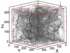
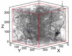
Figure 3. Streamlines for Re=0.31 with K=34 m/s (top) and for Re=152 with K=20 m/s (bottom) in 336 lu sub-sample ML-01.

There is a substantial reduction in the apparent hydraulic conductivity as the applied gradient increases to realistic field gradients (Figure 4). This suggests that under field conditions in the Biscayne aquifer, inertial flows and departures from the linear gradient-flow relation assumed in Darcy's law are likely to be common and important. Hydraulic conductivity and transmissivity measurements in such aquifers may commonly be reflective of inertial flow conditions and consequently are lower than they would be if these properties corresponded to the intrinsic permeabilities.

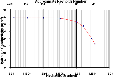
Figure 4. Effect of increasing gradient on apparent hydraulic conductivity for macroporous sample. Fitted Darcy-Forcheimer curve (solid line) and LBM simulation results (points).

SOLUTION OF TRANSIENT GROUND-WATER FLOW EQUATION WITH LBM

Although LBMs are effective pore-scale flow solvers, computation requirements make it unrealistic to consider solving aquifer-scale problems that involve matrix flow and transport through pore-scale simulation. Fortunately, there are two different approaches, briefly reviewed here, that can be adopted to simulate ground-water flow with LBM that are based on the macroscopic perspective inherent in Darcy's law and are not scale-dependent. One approach that utilizes a damping factor or force has been proposed in various forms and focuses on flow without considering solute transport. The literature describing these methods generally has not considered transient conditions nor internal source/sinks needed to simulate wells or recharge.

The second approach, which has rarely been considered previously in the literature (an exception might be Serván Camas [2007]), solves the transient ground-water flow equation using the well-established heat or diffusive mass transport analogy. We develop and demonstrate source/sink incorporation for that approach here.

The advantage of both of these methods for modeling flow and transport in karst comes from the linkage with the LBM's ability to solve the N-S and advection-diffusion equations in conduits within the porous matrix.

Damping Factor/Forcing Approach

Numerous papers have demonstrated the ability of LBM to characterize Darcian flow using an approach that damps out the inertial components of flow arising from the LBM's solution of the N-S equations with a damping factor or forcing related to the permeability of the domain [Dardis and McCloskey, 1998a,b; Freed, 1998; Martys, 2001; Kang et al, 2002; Guo and Zhao, 2002]. These approaches can solve a generalized N-S equation that includes the Brinkman-extended Darcy model (accounts for conduit/porous medium boundary conditions) and non-linear drag often represented by the Forchheimer equation. Following Freed [1998], Kang et al [2002] presented a similar model but also incorporated non-uniform grid spacing and used the model to draw conclusions about relative fracture/matrix permeabilities that justify the use of discrete fracture models that ignore matrix effects. The approach of Dardis and McCloskey [1998a,b] is described in more detail below; improved methods are in review.

In accordance with Darcy's law, the flow of fluid in a porous medium is proportional to the medium's permeability. Dardis and McCloskey [1998a,b] introduced a damping parameter 0 < n_s < 1, along with a new step in the LBM procedure to damp momentum in proportion to n_s. The n_s term can be a function of x, n_s = n_s(x), which allows simulation of heterogeneous porous media. If n_s = 0, the porous media step has no effect, and the process reduces to the usual free-fluid LBM. If n_s = 1, however, then flow is completely eliminated. The porous media step is applied only to the fluid component, not solute or heat components.

Dardis and McCloskey [1998a,b] indicated that the permeability k of a medium with damping factor n_s could be computed as

,

(5)

where n is the kinematic viscosity of the fluid phase. This has led to misunderstanding in the past because k is a medium property and should not depend on viscosity. In this particular macroscopic porous media approach, the viscosity no longer retains it normal meaning but instead, along with n_s, determines k in lattice units according to (5). Conversion to k in real units is straightforward:

,

(6)

where the L terms are the lengths of any comparable feature in physical and LBM units. Subsequent conversion to hydraulic conductivity is accomplished by multiplying by the physical fluid density and gravitational acceleration and dividing by the physical viscosity.

Figure 5 shows a simple conduit traversing a porous medium. A pressure gradient is applied across the domain from left to right. The conduit exerts a strong influence on the pressure field inside the domain. Dardis and McCloskey [1998a,b] and Kang et al. [2002] present similar results.

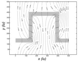
Figure 5. Pressure field in porous medium with conduit (gray).

Diffusion Equation Analogy Approach

There is a long tradition of simulating diffusion with LBM. It has recently been recognized that a less computationally intensive and more expedient approach to solving the transient ground-water flow equation

(7)

(where h, T, S and R represent the hydraulic head, transmissivity, storativity, and recharge respectively) in the LBM context is to solve it directly by exploiting its similarity to the diffusion or "heat" equation. One apparent advantage over standard explicit numerical methods is that the time step is not limited by the normal stability criterion [Wolf-Gladrow, 2000]. Also, unlike the damping methods, increasing T does not allow inertial effects, which can be considered a benefit in the context of a Darcy's law solver.

Other than specialized treatment of boundary conditions and source/sink terms, the only modification to the LBM technique involves truncating the equilibrium distribution function computation (3) (although models involving only 4 or 6 directions rather than 8 or 18 in 2- and 3-D, respectively, are viable for this approach [Wolf-Gladrow, 2000] and lead to substantial computational savings).

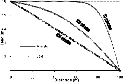
Below, we present two example LBM solutions of (7) that involve classic problems that have analytical solutions. The first is based on a 1-D problem that appears in Wang and Anderson [1982] and considers a confined aquifer bounded by two constant-head reservoirs (Figure 6). The aquifer is l=100-m long, has a T of 0.02 m² min^-1, and a storativity of 0.002. The head is initially uniform at 16 m (i.e., the initial condition is h|_x,0 = 16 m) and drops to 11 m at x = 100 at time 0 (i.e., the boundary conditions are h₁ = h|_0,t = 16 m and h₂ = h|_100,t = 11 m).

Figure 6.  Transient ground-water flow problem with two reservoirs (from Wang and Anderson, 1982).

We solve the problem and present the results relative to the analytical solution in Figure 7 below. The LBM results are excellent.

Figure 7. Comparison of LBM with analytical solution for transient reservoir problem.

The second test problem involves a pumping well in an infinite domain that is governed by the Theis well function. This test problem can be used to verify the LBM solution of the transient equipotential field (drawdown curve) in a 2-D aquifer with recharge/discharge. We use consistent LBM space and time units of "lu" (lattice length units) and "ts" (lattice time steps) in this case. Figure 8 shows drawdown as a function of time for a confined aquifer with T=1.0 lu²/ts and relaxation parameter equal to 0.95 ts, which gives the hydraulic diffusivity equal to 0.15 lu²/ts. The 50 lu × 50 lu domain is initialized with uniform head of 1 lu. The pumping well is set in the center (25, 25) and was pumped at a constant rate of 0.003 lu³/ts. Drawdown is measured 7 lu from the pumping well.

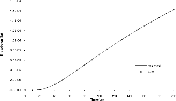
Figure 8. Well drawdown as a function of time; consistent LBM units.

There is a rich variety of possibilities for development of this method that need to be investigated. In particular, we have considered only quasi-3-D models and isotropic hydraulic conductivity so far.

The benefits of these macroscopic porous media approaches for karst ground-water flow simulation are substantial. First, they raise LBM from primarily a pore-scale N-S solver with computational limitations when field- and regional-scale simulations are required, to a standard ground-water flow solver applicable at any scale. Second, the spatial transition between the Darcy's law simulation and the full N-S solution in conduits is more straightforward than it is in other conduit/matrix models because the same algorithm underlies all of the computational domain, and switching between the different solutions involves only switching between n_s = 0 or n_s > 0 or between the two forms ((2) and (3)) of the equilibrium distribution function.

SOLUTE TRANSPORT FOR MACROSCOPIC POROUS MEDIA USING LBMs

The combination of the solute transport and Darcy's law capabilities of LBM discussed so far makes many types of simulations possible. One important characteristic of solute and heat transport in porous media is not addressed by simply combining these capabilities; unlike diffusion, dispersion under flow conditions in a porous medium is anisotropic. Zhang et al [2002a,b] and Ginzburg [2005] have introduced LBMs to simulate anisotropic dispersion. The approach of Zhang et al. [2002a,b] is described more fully and used in the examples below.

The dispersion tensor, D_ab, is given by Zhang et al [2002a,b]

,

(8)

where d_ab is the Kronecker Delta, G_L and G_T are the longitudinal and transverse dispersivities, respectively, (d_ab = 1 for a = b), and u_a and u_b are the are the a and b components, respectively, of the velocities. This equation is solved at each node. The dispersion tensor components D_xx, D_yy, D_xy and D_yx in terms of directional relaxation parameters, t_a, are expressed as [Zhang et al, 2002a,b]:

.

(9)

Given the dispersion tensor, these equations are inverted to solve for relaxation times that are subsequently used at each node in the model. To ensure mass conservation, Zhang et al [2002a,b] used a weighted summation of the particle distribution function as shown below to compute the density (concentration), r_s, of species subjected to the anisotropic dispersion:

,

(10)

where the weighting factors are represented by w_a and i represents a summation index.

Anisotropic dispersion of a solute plume moving at an angle to the main coordinate axes is shown in Figure 9. The longitudinal to transverse dispersivity ratio is 5:1 and the results compare well to the analytical solution.

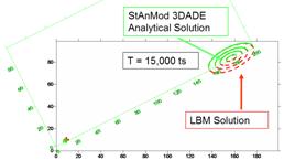
Figure 9. Anisotropic dispersion of 2-D solute plume (dashed contours) compared to the analytical solution (solid). G_L = 0.5, G_T = 0.1 lu. Flow unaligned with coordinate axes.

Incorporating this modification and combining it with the ground-water flow solvers discussed above yields an LBM ground-water flow simulator and a tightly coupled anisotropic dispersion ADE solver comparable to a number of available finite difference/finite element models. The new LBM ground-water/transport model inherits at least one exceptional capability from its foundation however-it can accurately simulate flow and transport in large conduits or fractures that may involve higher Reynolds number flows and associated eddy mixing.

We present one example that illustrates the power of the combination of processes that can be simulated. In Figure 10, a heterogeneous porous medium is cut by a conduit. A solute pulse is applied at the left boundary that quickly fills the conduit and begins invading the porous medium, particularly in zones of higher hydraulic conductivity such as the light colored areas above and left of center and at the lower right. The domain is then flushed with solute-free water. Clear "mushroom cap" plumes of solute-free water develop in the conduit illustrating the eddy-mixing phenomenon. Flushing of the conduit will be complete long before the adjacent porous medium is flushed. We expect this type of behavior in karstic aquifers and existing models offer less appropriate approximations.

Figure 10. Model domain (left) showing conduit (white) in porous medium of variable permeability (proportional to whiteness), solute invasion into porous medium, and eddy mixing in conduit (center). Periodic top and bottom boundaries account for appearance of solute in upper right. Breakthrough curve for domain (right) is complex and cannot be well-fitted with standard advection-dispersion model.

FUTURE APPLICATIONS

One of the main challenges in karst hydrology is characterizing/modeling the complex geometry present at many scales within karst aquifers and their macropore and conduit systems. Data for use in models proposed here can be obtained at different scales through thin sectioning of rock, imaging of hand- to body-sized specimens via digital photography or tomography, borehole televiewers or cross-hole tomography, ground penetrating radar, and traditional aquifer tests. Identification and characterization of macropore and conduit zones are logical next steps for enhancing understanding of karst aquifers and are active research areas [e.g., Cunningham et al., 2006].

We have competed preliminary work at the 1-m scale, based on borehole imagery from the Biscayne aquifer. In our approach, a borehole image is subject to thresholding to separate it into macropores and rock. Then the 3-D information available from the image is reconstituted by extracting the coordinates and presence or absence of rock at each pixel on the borehole wall. Variograms for the 3-D data are computed and simulation of 3-D rock is possible. Figure 11 shows a preliminary example of the potential of this method.

Figure 11. Left: Borehole televiewer image from 8-inch (~20 cm) diameter USGS borehole (G-3849) and thresholded 3-D data. (Photo by Michael Wacker, USGS). Right: Two simulations of 3-D rock based on borehole image variogram.

Suitable data from large caves are also available. Highly specialized dive teams have collected geometrical data from karst aquifers near Talahassee, Florida. Figure 12 shows a portion of the cave system that discharges to Wakulla Spring based on these data. Such data would be combined with traditional data on the properties of the surrounding aquifer to provide input for the combined LBM aquifer-conduit model.

CONCLUSION

LBMs offer solutions to challenges facing modelers of karst aquifer hydraulics and solute transport. Inertial flows expected when the Reynolds number is high enough and their effect on apparent hydraulic properties and solute transport can be simulated. Integration with LBM-based transient ground-water flow and anisotropic dispersion solvers may offer better solutions for karst problems.

 

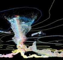
Figure 12. Geometry of Wakulla Spring viewed from below ground surface. Digital Wall Mapper data (courtesy Dr. Barbara Am Ende).

REFERENCES

Alvarez, P.F., 2007, Lattice Boltzmann modeling of fluid flow to determine the permeability of a karst aquifer. M.S. thesis, Florida International University, 96 pp.

Anwar, S., Cortis, A., and Sukop, M.C., 2008 (In press), Lattice Boltzmann simulation of solute transport in heterogeneous porous media with conduits to estimate macroscopic Continuous Time Random Walk model parameters. Progress in Computational Fluid Dynamics.

Bardsley, K.J., Anwar, S., and Sukop, M.C., 2006, Simultaneous heat and solute transport modeling of ground-water with lattice Boltzmann methods. CMWR XVI - Computational Methods in Water Resources, XVI International Conference, Copenhagen, Denmark , June 19-22

Bhatnagar, P.L. Gross, E.P., and Krook, M., 1954, A model for collision processes in gases. I. Small amplitude processes in charged and neutral one-component systems. Physics Review, 94, 511-525

Birk, S., Liedl, R., Sauter, M., and Teutsch, G., 2003, Hydraulic boundary conditions as a controlling factor in karst genesis: A numerical modeling study on artesian conduit development in gypsum. Water Resources Research 39 (1), 1004, doi:10.1029/2002WR001308.

Cunningham, K.J., Wacker, M.A., Robinson, E. Dixon, J.F., and Wingard, G.L., 2006, A cyclostratigraphic and borehole-geophysical approach to development of a three-dimensional conceptual hydrogeologic model of the karstic Biscayne Aquifer, southeastern Florida. U.S. Geological Survey Scientific Investigations Report 2005-5235, 69 p., plus CD.

Dardis, O., and McCloskey, J., 1998a, Permeability porosity relationships from numerical simulations of fluid flow. Geophys. Res. Let., 25, p. 1471-1474.

Dardis, O., and McCloskey, J., 1998b, Lattice Boltzmann scheme with real numbered solid density for the simulation of flow in porous media. Phys. Rev. E., 57, (4), p. 4834-4837.

Freed, D.M., 1998, Lattice Boltzmann method for macroscopic porous media modeling, Int. J. Modern Phys. C 9, p. 1491-1503

Ginzburg, I., 2005, Equilibrium-type and link-type lattice Boltzmann models for generic advection and anisotropic-dispersion equation. Adv. Wat. Resour., 28(11), p. 1171-1195.

Ginzburg, I., and d'Humières, D., 2003 Multireflection boundary conditions for lattice Boltzmann models Phys. Rev. E 68, 066614

Guo, Z., and Zhao, T.S., 2002, Lattice Boltzmann model for incompressible flows through porous media, Phys. Rev. E 66, 036304

Kang, Q., Lichtner, P.C., and Zhang, D., 2006, Lattice Boltzmann pore-scale model for multicomponent reactive transport in porous media. J. Geophys. Res. 111, B05203, doi:10.1029/2005JB003951

Kang Q., Zhang, D., and Chen, S., 2002, Unified lattice Boltzmann method for flow in multiscale porous media Phys. Rev. E 66 (5): 056307 

Li, H., Pan, C., and Miller, C.T., 2005, Pore-scale investigation of viscous coupling effects for two-phase flow in porous media. Phys. Rev. E 72, 026705

Martys, N.S., 2001, Improved approximation of the Brinkman equation using a lattice Boltzmann method. Phys. Fluids, 13(6), p. 1807-1810

Pan, C., Hilpert, M., and Miller, C.T., 2004, Lattice-Boltzmann simulation of two-phase flow in porous media. Water Resour. Res., 40, W01501, doi:10.1029/2003WR002120.

Pan, C., Luo, L.-S., and Miller, C.T., 2006, An evaluation of lattice Boltzmann schemes for porous medium flow simulation, Computers & Fluids 35(8/9), p. 898-909

Serván Camas, B., 2007, Saltwater intrusion simulation in heterogeneous aquifer using Lattice Boltzmann method, M.S. Thesis, Louisiana State University, 77 pp.

Sukop, M. C., and Or, D., 2004, Lattice Boltzmann method for modeling liquid-vapor interface configurations in porous media, Water Resour. Res., 40, W01509, doi:10.1029/2003WR002333.

Sukop, M.C., and Thorne, D.T., 2006, Lattice Boltzmann Modeling: An Introduction for Geoscientists and Engineers, Springer, Heidelberg- Berlin- New York. 172 pp.

Thorne, D.T., and Sukop, M.C., 2004, Lattice Boltzmann model for the Elder problem, In Proceedings of the XVth International Conference on Computational Methods in Water Resources (CMWR XV), June 13-17, 2004, Chapel Hill, NC, USA. C.T. Miller, M.W. Farthing, W.G. Gray, and G. F. Pinder Eds. Elsevier, Amsterdam.

Wang H.F., and Anderson, M.P., 1982, Introduction to Ground-water Modeling. W. H. Freeman and Company, San Francisco. 237 pp.

Watson, V., Painter, R., and By, T., 2003, Numerical simulation of flow and contaminant transport in a complex karst conduit. Society of Environmental Toxicology and Chemistry, 24th Annual Meeting in North America 9 - 13 November, Austin, Texas.

White, W.B., 2002, Karst hydrology: Recent developments and open questions. Engineering Geology 65, p. 85-105.

Wolf-Gladrow, D.A., 2000, Lattice-gas automata and lattice Boltzmann models: An introduction. Springer, Berlin. 308 pp.

Zhang, D.X., and Kang, Q. J., 2004, Pore scale simulation of solute transport in fractured porous media. Geophys. Res. Let. 31 (12): L12504.

Zhang X., Bengough, A.G. Crawford, J.W., and Young, I.M., 2002a, A lattice BGK model for advection and anisotropic dispersion equation, Adv Wat Resour 25, p. 1-8.

Zhang X., Crawford, J.W., Bengough, A.G., and Young, I.M., 2002b, On boundary conditions in the lattice Boltzmann model for advection and anisotropic dispersion equation. Adv Wat Resour 25, p. 601-609.