Uses and Importance of Long-Term Water-Level Data

U.S. Geological Survey Circular 1217

Previous Section: Box B 

Next Section: Box C

Return to Table of Contents

Return to Home Page

Water-level data are collected over various lengths of time, dependent on their intended use(s). Short-term water-level data are collected over periods of days, weeks, or months during many types of ground-water investigations (Table 1). For example, tests done to determine the hydraulic properties of wells or aquifers typically involve the collection of short-term data. Water-level measurements needed to map the altitude of the water table or potentiometric surface of an aquifer are generally collected within the shortest possible period of time so that hydraulic heads in the aquifer are measured under the same hydrologic conditions. Usually, water-level data intended for this use are collected over a period of days or weeks, depending on the logistics of making measurements at different observation-well locations.

Table 1. Typical length of water-level-data collection as a function of the intended use of the data.

Intended use of water-level data	Typical length of data-collection effort or hydrologic record required
	Days/weeks	Months	Years	Decades
To determine the hydraulic properties of aquifers (aquifer tests)
Mapping the altitude of the water table or potentiometric surface
Monitoring short-term changes in ground-water recharge and storage
Monitoring long-term changes in ground-water recharge and storage
Monitoring the effects of climatic variability
Monitoring regional effects of ground-water development
Statistical analysis of water-level trends
Monitoring changes in ground-water flow directions
Monitoring ground-water and surface-water interaction
Numerical (computer) modeling of ground-water flow or contaminant transport

In this report, the systematic collection of long-term water-level data is emphasized. Long-term data are fundamental to the resolution of many of the most complex problems dealing with ground-water availability and sustainability (Alley and others, 1999). As stated previously, significant periods of time—years to decades—typically are required to collect water-level data needed to assess the effects of climate variability, to monitor the effects of regional aquifer development, or to obtain data sufficient for analysis of water-level trends (Table 1).

Many of the applications of long-term water-level data involve the use of analytical and numerical (computer) ground-water models. Water-level measurements serve as primary data required for calibration and testing of ground-water models, and it is often not until development of these models that the limitations of existing water-level data are fully recognized. Furthermore, enhanced understanding of the ground-water-flow system and data limitations identified by calibrating ground-water models provide insights into the most critical needs for collection of future water-level data. Unfortunately, this second step of using ground-water models to help improve future water-level monitoring is rarely taken.

The uses and importance of long-term water-level data are more fully realized by examining actual case studies. Several are presented here to demonstrate the applicability of water-level data to a wide range of water-resource issues. These include the effects of ground-water withdrawals and other hydrologic stresses on ground-water availability, land subsidence, changes in ground-water quality, and surface-water and ground-water interaction.

Enhanced understanding of the ground-water-flow system and data limitations identified by calibrating ground-water models provide insights into the most critical needs for collection of future water-level data. Unfortunately, this second step of using ground-water models to help improve future water-level monitoring is rarely taken.

Ground-Water Development in the High Plains and Gulf Coastal Plain

In areas where aquifers are undergoing development, a long-term record of water-level measurements may encompass the transitional period between the natural and the developed state of the aquifer. Such records are invaluable in understanding and addressing problems that have developed in response to local and regional patterns of withdrawal, land use, and other human activities. This is demonstrated by the history of ground-water development of the High Plains aquifer and the Gulf Coastal Plain aquifer system (Figure 2).

Figure 2. Location of the High Plains aquifer and the Gulf Coastal Plain aquifer system.

The High Plains Aquifer

The High Plains is a 174,000-square-mile area of flat to gently rolling terrain that includes parts of eight States from South Dakota to Texas. The area is characterized by moderate precipitation but in general has a low natural-recharge rate to the ground-water system. Unconsolidated alluvial deposits that form a water-table aquifer called the High Plains aquifer underlie the region. During the late 1800’s, settlers and speculators moved to the plains, and farming became the major land-use activity in the area. Since that time, irrigation water pumped from the aquifer has made the High Plains one of the Nation’s most important agricultural areas.

Changes in ground-water levels in the High Plains aquifer are tracked annually through the cooperative effort of the USGS and State and local agencies in the High Plains region. Typically, water-level measurements are collected from about 7,000 wells distributed throughout the aquifer. Water-level measurements are made in the spring prior to the start of the irrigation season to provide consistency across the region. Information gathered in this multi-State cooperative effort reveals how changes in water stored in the aquifer vary from place to place depending on soil type, irrigation practices, recharge from precipitation, and the areal extent and magnitude of water withdrawals.

Over the years, the intense use of ground water for irrigation in the High Plains has caused major water-level declines (Figure 3) and decreased the saturated thickness of the aquifer significantly in some areas. For example, in parts of Kansas, New Mexico, Oklahoma, and Texas, ground-water levels have declined more than 100 feet. Decreases in saturated thickness of the aquifer exceeding 50 percent of the predevelopment saturated thickness have occurred in some areas. In other parts of the aquifer, such as along the Platte River in Nebraska, the recharge provided by the infiltration of excess irrigation water has caused ground-water levels to rise. The multi-State ground-water-level monitoring program has allowed all of these changes to be tracked over time for the entire High Plains region and has provided data critical to evaluating different options for ground-water management. This level of coordinated ground-water-level monitoring is unique among major multi-State regional aquifers.

Figure 3. Changes in ground-water levels in the High Plains aquifer from before ground-water development to 1997. (V.L. McGuire, U.S. Geological Survey, written commun., 1998.)

The Gulf Coastal Plain Aquifer System

The Gulf Coastal Plain aquifer system consists of a large and complex system of aquifers and confining units that underlie about 290,000 square miles extending from Texas to westernmost Florida, including offshore areas to the edge of the Continental Shelf. The Gulf Coastal Plain aquifer system represents a composite example of many of the issues for which long-term water-level data are collected and used. Water withdrawals from the aquifer system have caused lowering of hydraulic heads at and near pumping centers; reduced discharges to streams, lakes, and wetlands; induced movement of saltwater into parts of aquifers that previously contained freshwater; and caused land subsidence in some areas as a result of the compaction of interbedded clays within aquifers.

The Gulf Coastal Plain aquifer system represents a good example of the need to measure water levels in wells completed at different depths and in the context of a three-dimensional ground-water-flow system. For example, in order to simulate ground-water flow for the entire aquifer system, Williamson and Grubb (in press) subdivided the aquifer system into 17 regional aquifers and confining units, most of which are shown in the vertical section in Figure 4. Even this level of subdivision represents a very coarse subdivision of the aquifer system given its complexity and variability. Numerous more refined subdivisions of parts of the aquifer system for smaller scale studies have been made during the long history of ground-water studies in the region.

Figure 4. Aquifers and confining units and designation of layers in a regional model of the Gulf Coastal Plain aquifer system. (Modified from Williamson and Grubb, in press.)

The value of long-term water-level data for the Gulf Coastal Plain aquifer system is illustrated by briefly examining the history of ground-water development near three large cities (Memphis, Tennessee; Houston, Texas; and Baton Rouge, Louisiana) and by examining some fundamental changes in the regional ground-water-flow system.

The Gulf Coastal Plain aquifer system represents a good example of the need to measure water levels in wells completed at different depths and in the context of a three-dimensional ground-water-flow system.

Memphis, Tennessee

The Memphis aquifer (Memphis Sand) is the principal source of water for municipal, commercial, and industrial uses in the Memphis area of Tennessee. Pumpage increased from completion of the first well in 1886 until about 1974, when rates stabilized. Prior to development, the potentiometric surface of the Memphis aquifer is presumed to have been a smooth surface with a gentle slope to the west-northwest (Figure 5). Water-level data indicate that over the years a regional cone of depression has developed in the potentiometric surface of the aquifer, centered near downtown Memphis (Figure 6). As a result of ground-water withdrawals, the general direction of ground-water flow is toward the center of the regional cone of depression. Smaller cones of depression are superimposed upon this regional cone in areas heavily pumped by municipal and industrial wells.

Figure 5. Inferred potentiometric surface of the Memphis aquifer prior to ground-water development. The observation wells shown were selected for their early records away from initial pumping centers. (Modified from Criner and Parks, 1976.)

Water-level hydrographs for two selected wells through 1995 show the effects of long-term pumpage (Figure 7). One well (Figure 7A) is near the center of the regional cone of depression and has one of the longest nearly continuous records of water-level measurements in the United States. Between 1928 and 1975, the water level in this well declined about 70 feet and then stabilized as the pumping rates stabilized. A second well (Figure 7B) is east of the center of the regional cone of depression. Water levels in this well have declined steadily since records began in 1940, suggesting that the cone of depression continued to expand eastward for at least 20 years past the overall stabilization in pumping rates. Note that the seasonal fluctuation in water levels recorded in these observation wells is primarily a result of seasonal differences in water demand and pumping (as opposed to changes in aquifer recharge) and is much greater near the center of the cone of depression (Figure 7A) than in outlying areas (Figure 7B).

Figure 7. Declining water-level trends in two long-term observation wells in the Memphis area. Locations of wells are shown in Figure 6.

Long-term monitoring of water levels in the Memphis aquifer continues to provide essential information for management of this critical aquifer. As noted, monitoring is important not only near the major pumping centers but also in outlying areas.

Houston, Texas

Trends in ground-water withdrawals in the Houston, Texas, area are related to population and industrial growth, replacement of ground water by surface water as a source of supply in some parts of the area, and a shift from withdrawal for irrigation to public supply as a result of urban expansion. Ground-water withdrawals more than doubled every 20 years in the area during 1900–60 (Wood and Gabrysch, 1965). Ground water was the sole source of public-water supply for Houston until 1954, when surface water was introduced from the San Jacinto River. As a result of the increased use of surface water and reduced ground-water withdrawals, ground-water levels stabilized in the industrial district of Houston in the mid-1970’s and began to recover in 1977 (Figure 8A). However, ground-water withdrawals continued to increase to the north and west of Houston because of urban development. As a result, water levels in these areas continued to decline (Figure 8B).

Figure 8. Water-level trends in selected wells in the Houston area showing (A) stabilization and recovery of water levels in the industrial district and (B) declining water levels north and west of Houston. (Modified from Grubb, 1998.)

Extensive land subsidence has occurred in the greater Houston area as a consequence of the decline in ground-water levels. Long-term water-level measurements in the Houston area are invaluable indicators of the potential for subsidence. So long as hydraulic heads (indicated by water-level measurements) remain above previous minimum heads, the deformation of the aquifer is reversible. When hydraulic heads decline below previous lows, the structure of interbedded clay and silt layers may undergo significant rearrangement, resulting in irreversible aquifer-system compaction and land subsidence. In this low-lying coastal environment, as much as 10 feet of subsidence has increased the vulnerability of much of the area to flooding, caused permanent inundation of some areas, and activated faults causing damage to buildings, highways, and other structures. Subsidence to the east of Houston has been arrested as imported surface-water supplies have been substituted for ground-water pumpage, but the fast-growing areas to the north and west, which still depend largely on ground water, are subsiding in response to declining ground-water levels (Figure 9).

Figure 9. Relation between water-level trends and land subsidence in the Houston area. (Modified from Kasmarek and others, 1997;Coplin and Galloway, 1999.)

Baton Rouge, Louisiana

Trends in ground-water levels in the Baton Rouge area reflect growth in population and industry. Withdrawals increased more than tenfold from the 1930’s to 1970 and have since leveled off to some extent. In 1995, about 140 million gallons per day (Mgal/d) of ground water were pumped in the Baton Rouge area.

Sand layers at depths between about 400 and 2,800 feet are major aquifers in the Baton Rouge area. Locally, the aquifers are referred to by the general depth of the top of the aquifer in the area, for example, the “2,000-foot” sand. The effects of overall increases of withdrawals on ground-water levels, as well as of a shift in pumpage from shallower to deeper sands, are shown for wells in the industrial area of Baton Rouge in Figure 10.

Figure 10. Water-level trends in the Baton Rouge area, Louisiana, 1940–99. (Modified from Grubb, 1998.)

The hydrograph in Figure 10 for the shallower ground water is a composite of water levels in three wells monitored over the years in the “400-foot” and “600-foot” sands. During the early 1940’s to mid-1950’s, the “400-foot” and “600-foot” sands were the most heavily pumped aquifers in the Baton Rouge area, and pumpage reached a peak of 35 Mgal/d about 1942 (Kuniansky, 1989). The hydrograph indicates that, after reaching record water-level lows in the mid-1950’s, water levels (heads) in these aquifers rose steadily from the late 1950’s to 1990. During that period, deeper aquifers were developed, pumpage from the “400–600 foot” sands declined (to about 12 Mgal/d in 1990), and pumping centers became distributed over wide areas. Water levels again declined in the 1990’s as withdrawals from the shallow aquifers increased (pumpage was about 20 Mgal/d in 1995). Water-level declines in the well shown (well EB–870) were limited, however, because the pumping was less concentrated near that well location.

Prior to about 1920, pumpage from the “2,000-foot” sand was small (less than 0.5 Mgal/d) and had little effect on heads in the aquifer (Torak and Whiteman, 1982). Pumping increased sharply
to more than 10 Mgal/d after 1940 and has become redistributed in the Baton Rouge area as the locations of the major pumping centers have changed. A long-term hydrograph for well EB–90 (Figure 10) completed in the “2,000-foot” sand shows that, as water use from this deeper aquifer increased, heads in the aquifer continued to decline from 1940 to the 1970’s. After reaching a maximum rate of 44 Mgal/d in 1976, pumpage from the “2,000-foot” sand began to decline to about 32 Mgal/d by 1985, resulting in a slight recovery in heads. From 1985 to 1995, pumpage increased, and water levels in well EB–90 declined again in the 1990’s, albeit at a slower rate than before.

The large water-level (head) declines in the Baton Rouge area caused saltwater encroachment from the south in several of the sand aquifers (Figure 11). Long-term water-level monitoring is essential to continued understanding and forecasting movement of saltwater in the Baton Rouge area (as well as in other areas of the country, as discussed in later examples).

Figure 11. Saltwater encroachment in the “1,500-foot” sand aquifer moving toward pumping centers in the Baton Rouge area, Louisiana. A low-hydraulic-conductivity fault zone retards saltwater movement in the area. Nevertheless, saltwater has leaked through the fault zone in some areas in response to pumping. (Modified from Tomaszewski, 1996.)

The preceding examples for Memphis, Houston, and Baton Rouge illustrate how the history of ground-water development is reflected in long-term water-level records and how these records are essential to monitoring the effects of development and providing data needed for quantitative assessments of future management and development options. For all three metropolitan areas, individual long-term monitoring wells have provided valuable information about water-level trends at specific locations, but multiple wells are needed to track conditions in different aquifers and changes in cones of depression as pumping centers evolve. Furthermore, the examples show how information about ground-water withdrawals can be critical to the interpretation of water-level data.

Individual long-term monitoring wells have provided valuable information about water-level trends at specific locations, but multiple wells are needed to track conditions in different aquifers and changes in cones of depression as pumping centers evolve.

Information about ground-water withdrawals can be critical to the interpretation of water-level data.

Changes in Regional Ground-Water Flow

Measuring water level in observation well in Colorado. Photograph by Heather S. Eppler, U.S. Geological Survey.

As illustrated in the previous examples, more than 100 years of ground-water withdrawals have greatly altered ground-water conditions in the Gulf Coastal Plain aquifer system. As a result, there have been large-scale, regional changes in directions of horizontal flow, changes in vertical direction of flow between aquifers, increases in regional recharge to aquifers, and decreases in regional discharge from aquifers.

Ground-water withdrawals from deeper aquifers in the Gulf Coastal Plain aquifer system have caused a reversal of vertical-flow directions from upward to downward throughout thousands of square miles. This was evident locally for the Baton Rouge area by the crossing of the water-level hydrographs in Figure 10. That is, heads in the upper sands were lower than heads in the underlying “2,000-foot” sand prior to the early 1960’s, resulting in upward flow. As withdrawals shifted to the deeper aquifers, heads in the “2,000-foot” sand declined below those in the shallower sands, reversing the vertical direction of flow from upward to downward.

The relative changes in heads with depth and the magnitude and direction of vertical flow between aquifers are significant factors affecting future pumping lifts, base flow to streams, saltwater intrusion, and land subsidence. Such changes in an aquifer system typically are evaluated using computer model simulations. For example, the simulated widespread reversal of vertical-flow directions from predevelopment to 1987 for the upper part of the Gulf Coastal Plain aquifer system is shown in Figure 12. Model calibration and estimation of model accuracy required water levels measured at different depths before and after development and relied heavily on a compilation of water-level data collected by many prior studies throughout the region (Williamson and Grubb, in press).

Figure 12. Areas where vertical flow between uppermost aquifer layers reversed from upward under predevelopment conditions to downward by 1987, as simulated in regional model of Gulf Coastal Plain aquifer system. (Modified from Grubb, 1998.)

Drought Monitoring in Pennsylvania

More than 40 million people in the United States supply their own drinking water from domestic wells. Many of these wells are shallow and vulnerable to extended droughts. Yet, relatively few observation wells are measured regularly to provide an indication of the response of ground water to climatic conditions. Wells for such purposes are needed in relatively undeveloped recharge areas where water-level fluctuations primarily reflect climatic variation rather than ground-water withdrawals or human-induced recharge. The timeliness of water-level data also is a critical factor. Most wells are measured monthly or less frequently. Even if wells are equipped with a digital water-level recorder, the data must be retrieved and processed before they are available. As a result, available water-level data commonly lag behind current conditions from one to several months.

Continuous collection, processing, and transmittal of water-level data by satellite and other telecommunication methods are increasingly being used to display real-time ground-water conditions on the Internet. The need for this type of information became evident during the summer of 1999, when drought in the Eastern United States resulted in drought declarations or water restrictions in 15 States. Following a relatively dry spring and summer, rainfall from several large storms, including Tropical Storm Dennis and Hurricane Floyd, occurred in many of these States during the months of August and September 1999. After each storm, questions arose about whether water restrictions should be lifted. Each time, information on ground-water conditions was sought to help provide a complete picture of the drought conditions. The information typically was limited and not current. The State of Pennsylvania was an exception.

Continuous collection, processing, and transmittal of water-level data by satellite and other telecommunication methods are increasingly being used to display real-time ground-water conditions on the Internet.

In 1931, in response to concerns about ground-water-level declines caused by the drought
of 1930, a statewide well network was established in Pennsylvania to monitor water-level fluctuations. Today, this network consists of about 50 wells (Figure 13) operated by the USGS in cooperation with the Pennsylvania Department of Environmental Protection. The primary purpose of the observation-well network is to monitor ground-water conditions for indications of drought. The Pennsylvania Emergency Management Council uses data from the wells when categorizing counties for a drought declaration. Currently (2001), water levels for about 80 percent of the network wells are transmitted by satellite telemetry and displayed on the USGS Web pages for Pennsylvania.

Figure 13. Location of drought-index wells and ground-water-level conditions in Pennsylvania in July 1999.

An observation-well network of 23 wells established in 1973 provides additional spatial
resolution for ground-water conditions in Chester County, Pennsylvania (Schreffler, 1997). The Chester County network was established through a cooperative agreement between the Chester County Water Resources Authority and the USGS. The wells are distributed throughout the county in different geographic and geologic settings. A water-level hydrograph for a well that is in both the statewide network and the Chester County network is shown in Figure 14 for water years 1998 and 1999.

Figure 14. Hydrograph for drought-index well in Chester County, Pennsylvania, showing water levels from October 1997 to September 1999, compared to established monthly drought-warning and drought-emergency water levels. (D.W. Risser, U.S. Geological Survey, written commun., 2000.)

Data from the Pennsylvania network were used by the State to help respond to the 1999 drought. When drought emergency was declared in 55 Pennsylvania Counties in July 1999, one-third of the State’s network wells had record-low seasonal levels. The Governor was able to note that “(ground-) water levels we’re seeing today—in the middle of summer—are on par with levels we would see in September or October…Groundwater levels typically won’t begin to recharge until the leaves are off the trees and we get sustained rains in the fall” (Pennsylvania Department of Environmental Protection, news release, July 20, 1999).

Estimation of High Ground-Water Levels in Massachusetts and Rhode Island

Statistical evaluations of water-level data collected for one or more decades can be used
to estimate future high, low, and medium or “normal” water levels. The accuracy of these water-level estimates improves as the length of record increases.

In populous areas of coastal Massachusetts and Rhode Island, water levels normally change by several feet annually but can change by as much as 20–30 feet (Socolow and others, 1994). This potentially wide range of ground-water fluctuation can result in adverse effects to home and building construction. Estimates of the maximum (highest) probable ground-water levels are needed to assess the likely chances for basement flooding, damage to building foundations due to increased hydrostatic pressure, and the potential failure of septic tanks and leach fields in unsewered areas (Figure 15).

Figure 15. Sketch showing effects of unanticipated high ground-water-level fluctuations on housing structures. (Modified from Socolow and others, 1994.)

To address this problem, USGS hydrologists in Massachusetts developed a technique to estimate the potential maximum ground-water level at a site where only a single measurement of water level may be available (Frimpter, 1980; Frimpter and Fisher, 1983). The technique uses a water-level measurement taken at the site of interest in combination with information on the concurrent water level and statistical distribution of water levels in a long-term observation well chosen as an “index” well and information on the range of water-level fluctuations at observation wells in similar geologic and hydrologic settings. The index well should be unaffected by pumping and other human-induced hydraulic stresses, completed in the same geologic material as that underlying the site of interest, and located in a similar topographic setting. Moreover, the index well must have a hydrologic record sufficiently long to provide for a statistically based determination of the range in water-level fluctuations.

In Massachusetts, water-level measurements from nine index wells having 16–28 years of hydrologic record and about 160 wells having shorter periods of record were used to map five zones of different ranges in annual water-level fluctuations in glacial sand, gravel, and till deposits that underlie Cape Cod (Frimpter and Fisher, 1983). Subsequent application of the technique in Rhode Island was limited by the distribution of suitable index wells (Socolow and others, 1994). Approximately 15 wells completed in glacial sand and gravel deposits and having hydrologic records that span the period between 1946 and 1989 were determined to be of suitable length for use as index wells. Because of relatively short (generally less than 5 years) or discontinuous hydrologic records, however, no suitable index wells were identified among the observation wells available in the till deposits of Rhode Island.

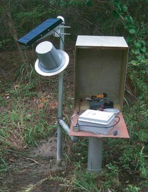Water well instrumented for satellite transmission and real-time reporting on the Internet. Photograph by William L. Cunningham, U.S. Geological Survey.

Ground-Water and Surface-Water Interaction in Oregon

The effect of ground-water development on surface-water resources is increasingly a focus of ground-water studies (Winter and others, 1998). Yet, stream-gaging and water-level monitoring networks are rarely jointly designed with this use of data in mind. The upper Deschutes Basin, an area of rapid population growth in central Oregon, provides an example of the importance of combined ground-water and surface-water data.

Quantitative assessments of the ground-water system and its interaction with surface-water resources of the upper Deschutes Basin have been crucial in supporting resource-management decisions in the basin. Surface-water resources in the area have been closed by the State to additional appropriation for many years. Thus, virtually all new development in the basin must rely on ground water as a source of water supply.

The effect of ground-water development on surface-water resources is increasingly a focus of ground-water studies. Yet, stream-gaging and water-level monitoring networks are rarely jointly designed with this use of data in mind.

Figure 16. Location of field-located wells in upper Deschutes Basin study area, Oregon. (Modified from Caldwell and Truini, 1997; Gannett and others, 2001.)

Figure 17. Plot showing location of measured wells in upper Deschutes Basin, Oregon, and times of water-level measurement, 1977–98. Measurements from long-term observation wells are shown in red. (M.W. Gannett, U.S. Geological Survey, written commun., 2000.)

Recharge resulting from leakage from streams and irrigation canals and from on-farm irrigation losses greatly exceeds recharge from precipitation in the dry plains of the eastern and central part of the basin. Examples of combined use of water-level and stream-gaging data to provide information on the streams and canals as a source of recharge to the basin are shown in Figures 18 and 19. Understanding these relations is critical to quantitative modeling of the basin hydrologic system.

Figure 18. Hydrographs of the stage of the Deschutes River at Benham Falls and water levels in wells 500 and 5,000 feet from the river. (Gannett and others, 2001.)

Figure 19. Relation between the static water level in a well in upper Deschutes Basin, Oregon, and the stage in an irrigation canal about one-half mile away. Although over 600 feet below land surface, the water level in the well starts to rise shortly after the canals start flowing and starts to drop soon after they are shut off for the season. The water level also responds to periodic short-term operation of the canal. (Gannett and others, 2001.)

Figure 18 shows hydrographs of the stage of the Deschutes River at Benham Falls and water levels in wells 500 and 5,000 feet from the river. This is a reach in which the river loses about 100 cubic feet per second into permeable lava. Stream-gaging data show that the rate of loss is proportional to the river stage. The well closer to the river is near the gaging station. The well farther from the river is about 4 miles downstream from the station. Water levels in both wells respond to changes in river stage, and the effect is attenuated and delayed with distance from the river.

Figure 19 shows the relation between the static water level in a 690-foot well and the stage in an irrigation canal about one-half mile away. Canal leakage is a significant source of local recharge in the more arid areas of the basin. The canals commonly operate during the irrigation season from April through the beginning of October and also are used periodically at other times to fill stock ponds and other storage facilities. Isotopic evidence (Caldwell, 1998) substantiates that the canal (and possibly the Deschutes River from which this and other canals originate) is likely the predominant source of water to this well and other wells in areas traversed by irrigation canals.

Wetland Hydrology in Michigan

Wetlands provide many beneficial functions such as flood control, water-quality modification, and habitat for wildlife. Increasingly, artificially constructed wetlands are used in flood mitigation and for treatment of acid-mine and wastewater discharges. While they are often thought of only in the context of surface water, most wetlands are ground-water-discharge areas. The storage of water is crucial to wetland ecology and hydrologic functions (Carter, 1996). In many wetlands, the depth to ground water and ground-water-level fluctuations largely control the capacity for water storage. Moreover, ground-water levels are often important in maintaining the physical and chemical conditions in the root zone that promote healthy and stable growth of wetland plants (Hunt and others, 1999).

Because of the complex interaction between surface and ground water in wetlands, ground-water discharge and storage commonly are difficult components of the wetland hydrologic system to characterize. Restoration of former wetlands or construction of functional artificial wetlands requires knowledge of ground-water-flow gradients and the natural range in seasonal fluctuations in the water table. One example of the need for water-level data to assess the efforts required to restore a wetland is highlighted by a project underway in the Seney National Wildlife Refuge, in the Upper Peninsula region of Michigan (Figure 20). Wetlands in the wildlife refuge were drained in 1912 in a failed attempt to convert the land to agricultural use. Research began in 1998 to evaluate the potential for restoration of the wetland ecosystem in approximately 33,500 acres of the refuge (Sweat, 2001). Engineering controls will be used to rehydrate wetland soils and increase the altitude of the water table. However, the natural range of ground-water-level fluctuation within the wetland area is not known. If ground-water levels decline significantly or are subject to severe seasonal fluctuations, wetland ecosystems can be disrupted and the function and sustainability of the wetland can be impaired.

Figure 20. Ground-water and surface-water observation stations in the watershed management area of the Seney National Wildlife Refuge wetlands, in the Upper Peninsula region, Michigan. Photograph shows hydrologists making flow measurements in a perennially flooded pool in the wetland area at the refuge. (Courtesy of “People, Land, and Water,” October 1998, published by U.S. Department of the Interior, Washington, D.C.)

Because available water-level data were not sufficient to determine seasonal trends and the range of ground-water-level fluctuations, investigators have installed 11 long-term ground-water observation wells and 7 combined ground-water and surface-water gaging stations (Figure 20). Data collected at these sites will be used to assess the average range of water-level fluctuations under the existing conditions, to determine how much ground-water levels need to be raised to support wetland ecologic functions, and to manage wildlife habitat and flood control in a perennially flooded pool in the wetland.

Downloading data from automatic water-level recorder. Photograph by Michael D. Unthank, U.S. Geological Survey.

Relevance of Water-Level Data to Ground-Water Quality Issues

The role of water-level data in the investigation of ground-water quality or contamination problems is sometimes underappreciated. To a large degree, predictions about the speed and direction of movement of ground-water contaminants are based on determination of the gradient (slope) of the water table or potentiometric surface in the affected aquifer. While the data needed for these determinations typically are obtained by synoptic water-level surveys, longer term water-level measurements are often needed to develop an understanding of how ground-water contaminants migrate from their sources through the ground-water system. For example, an examination of water-level hydrographs and graphs of contaminant concentrations over time may reveal a relation between the occurrence of event-related or seasonal changes in ground-water recharge and fluctuations in the contaminant concentrations.

Increasingly, computer-based solute-transport models are used to simulate subsurface migration and behavior of ground-water contaminants. Water-level data of sufficient duration and frequency of measurement are needed to calibrate and evaluate the reliability of the flow component of these models before realistic simulations of contaminant transport can be made.

Many ground-water-quality problems develop over long periods due to human-induced changes
in hydraulic heads and resultant changes in the dynamics of a ground-water-flow system. Degradation of freshwater aquifers by the intrusion of saline water is a particularly common ground-water-quality problem of this type.

The use of long-term water-level data to address saline-water intrusion is presented in two examples here. These are followed with an example related to concerns about ground-water degradation from residential development.

The role of water-level data in the investigation of ground-water quality or contamination problems is sometimes underappreciated.

Saline Water Intrusion in New Jersey

The relation between the intrusion of saline water and declining hydraulic heads due to extensive aquifer development is well illustrated by the aquifers in the Coastal Plain of New Jersey (Lacombe and Rosman, 1997). Since the 1800’s, the principal source of public-water supply in the Coastal Plain of New Jersey has been ground water obtained from wells in 10 major confined aquifers. The aquifers are arranged in a dipping, layered ground-water system similar to that of the Gulf Coastal Plain aquifer system. Because of large ground-water withdrawals, regional cones of depression have developed in each of the aquifers. By 1978, the potentiometric surfaces of most of the aquifers had been lowered below sea level, and natural flow directions in some areas were reversed. Consequently, saline water that is naturally present in the deeper parts of the aquifers was induced to migrate toward pumping centers, and chloride and dissolved-solids concentrations increased significantly in parts of these aquifers.

As an example, pumping by public-supply wells completed in the Upper Potomac-Raritan-Magothy aquifer near the New Jersey coastline resulted in a decline in hydraulic heads to more than 40 feet below sea level (Schaefer and Walker, 1981). The development of this large cone of depression in the potentiometric surface in the aquifer also resulted in the landward reversal of ground-water flow and migration of saline water. Throughout the 1970’s, ground water in parts of the aquifer became progressively degraded by sharply rising chloride concentrations, as shown for the Union Beach well field in Figure 21. Although pumping was curtailed in the 1980’s, degradation of the aquifer by saline water was sufficiently extensive that the well field was later abandoned and replaced by wells farther inland.

Figure 21. Relation between reductions in heads from pumping and chloride concentrations in the Upper Potomac-Raritan-Magothy aquifer, New Jersey, 1977. Chloride concentrations shown in the graph are a composite of concentrations in water samples from wells screened at about the same depth in the Union Beach well field. (Modified from Schaefer and Walker, 1981.)

Because of the continued potential threat of degradation of the freshwater parts of the aquifers, ground-water withdrawals are carefully monitored and regulated by the New Jersey Department of Environmental Protection (NJDEP). In addition, the NJDEP and USGS have developed a cooperative program to monitor changes in water levels and chloride concentrations at 5-year intervals in each of the confined aquifers. As part of this monitoring program, water-level hydrographs are prepared from continuous measurements collected in 99 long-term observation wells and used to assess seasonal trends in ground-water recharge and storage. Water-level measurements are made in approximately 1,000 additional observation wells and used to construct potentiometric maps showing any significant changes in the size of the cones of depression developed in the aquifers. Water samples are collected from selected observation wells for analysis of chloride and dissolved-solids concentrations, and these data are compiled to monitor changes in the relation between hydraulic heads, ground-water-flow directions, and ground-water quality. Using this combined water-level and water-quality monitoring program, the NJDEP can evaluate the effects of water-management decisions on the aquifers and carefully monitor the improvement or further degradation of water quality in the aquifers.

Upwelling of Saline Water in Utah

Chloride contamination also can occur in noncoastal areas where the freshwater aquifer is invaded by saline water or brines upwelling from deeply buried sedimentary rocks. Spangler and others (1996) documented an example of this problem in a study of the quality of water in the Navajo aquifer in southeastern Utah.

The Navajo aquifer, composed of the Entrada and Navajo Sandstone formations, is one of several aquifers separated by confining units within a large sedimentary basin that underlies San Juan County, Utah (Figure 22). Within the basin, the top of the Navajo aquifer averages about 550 feet below land surface, and the thickness of the aquifer generally ranges from 750 to 1,000 feet. The Navajo aquifer is recharged mainly by infiltration where the sandstones crop out at the surface along several mountain ranges that surround the basin. The Navajo aquifer is confined above by the Wanakah Formation and below by the Chinle-Moenkopi Formation. Artesian pressures are so great in parts of the aquifer that ground water discharges naturally at the land surface from open, flowing wells.

Figure 22. Geologic section showing the stratigraphic relations and movement of ground water between the Navajo aquifer, upper Paleozoic aquifer, and other major aquifers and confining units, San Juan County, southeastern Utah. (Modified from Spangler and others, 1996.)

Much of the sedimentary basin that contains the Navajo aquifer has been explored and developed for oil and gas. Several oil fields were developed in the basin in the 1950’s, and exploration and production generally have increased since then. The main oil-producing zones in the basin are in carbonate rocks of the Paradox Formation, at depths ranging from 5,000 to 6,000 feet below land surface. Over time, as oil was extracted and oil-field pressures declined, the technique of water flooding—the injection of freshwater from alluvial aquifers along the San Juan River to flush residual oil—was used to boost production in the Paradox Formation oil wells. This practice began in the late 1950’s and continues to the present. Brine water, obtained from the Paradox Formation as a by-product of the water flooding and oil recovery process, was reinjected into deep wells completed in the oil-producing zones for disposal.

Water-quality problems associated with increased chloride concentrations in wells drilled into the Navajo aquifer began to be reported in the 1950’s. A review of historical water-level records indicated that hydraulic heads in the Navajo aquifer had declined by as much as 178 feet since the early 1950’s because of increased development. The decline in hydraulic heads in the Navajo aquifer had resulted in an increased upward hydraulic gradient between the upper Paleozoic aquifer and Navajo aquifer (Figure 23). This indicated that ground water from the upper Paleozoic aquifer could provide recharge to the Navajo aquifer in locations where the Chinle Formation confining unit was breached by fractures or by improperly sealed wells.

Figure 23. Potentiometric map of the Navajo aquifer showing locations of wells used for water-level measurements and the inferred area of upward ground-water flow from the upper Paleozoic aquifer, San Juan County, southeastern Utah. (Modified from Spangler and others, 1996.)

The information from historical water-level measurements was used to guide water-quality sampling needed to identify the source of the chloride contamination in the Navajo aquifer. Water samples were collected from wells completed in the Navajo aquifer, the upper Paleozoic aquifer, the Paradox Formation, and other deep aquifers (Spangler and others, 1996). Samples of the brine water being reinjected at producing oil wells also were collected. Detailed chemical analyses of these water samples indicated that the degradation of water quality in wells completed in the Navajo aquifer was caused primarily by the upwelling and mixing of saline water from the upper Paleozoic aquifer. The brine water reinjected into the Paradox Formation was determined to be an unlikely source of the chlorides in the Navajo aquifer. The oil and gas production activities may have contributed indirectly to the water-quality problem, however, as a review of well-construction logs identified over 200 active and abandoned oil wells that may be inadequately cased or sealed. These wells could provide conduits by which ground water migrates upward from the upper Paleozoic aquifer and intermingles with ground water in the Navajo aquifer.

Effects of Residential Development in Montana

The early stages of land or aquifer development is an opportune time to establish a combined water-level and water-quality monitoring network that can define baseline conditions and track important changes with time in the quantity and quality of the resource. Examples are provided for the Gallatin and Helena areas in southwestern Montana, which are among many parts of the Western United States where rapid changes in land development have the potential to affect ground-water resources.

The Gallatin Valley is an intermontane basin that consists of an alluvial plain flanked by higher elevation benches (Figure 24). The alluvial plain is used primarily for irrigated agriculture and the benches for dryland farming. In recent years, residential and commercial development has replaced considerable areas of farmland on both the alluvial plain and the benches. Much of the population increase has been outside of established cities and towns, in areas where each home has its own well and septic system. The residential development has raised concerns regarding the potential effects of infiltrating septic wastewater on the quality of ground water. In response, the Gallatin Local Water Quality District (GLWQD) was established in 1995, and efforts were undertaken to monitor the quality of ground water and surface water.

Figure 24. Perspective block diagram of the Gallatin Local Water Quality District, Montana, showing areas of urban and residential development. (Modified from Kendy, 2001.)

Long-term water-level measurements are needed to provide information on trends or variations in annual recharge that may affect either the amount of dilution or the additional loads of contaminants that may be introduced to the ground-water system from the septic wastewater. Since the late 1940’s, periodic surveys have been made of water levels in the valley, but only two wells have been measured consistently from year to year. Both wells are near or within the flood plain of the Gallatin River. Water levels in the two wells primarily represent recharge from the river or from local diversions of river water for irrigation. Little water-level monitoring has been done for the aquifers underlying the benches (Kendy, 2001). To help address these issues, in 1997 the USGS designed a long-term water-level monitoring network in cooperation with the GLWQD that consists of 101 wells. An attempt was made to include as many previously monitored wells as possible and to expand the network to represent all developed aquifers in the GLWQD.

The early stages of land or aquifer development is an opportune time to establish a combined water-level and water-quality monitoring network that can define baseline ground-water conditions and track important changes with time in the quantity and quality of the resource.

Like Gallatin Valley, the Helena, Montana, area has experienced marked growth in recent years. Public concerns about depletion or contamination of ground water in the bedrock areas surrounding the Helena Valley led to a hydrologic study by the USGS in cooperation with the Lewis and Clark County Water Quality Protection District (Thamke, 2000) that is similar to the study described previously for the Gallatin area.

Monthly measurements of water levels in 112 wells from 1993 to 1998 were an important part of the Helena bedrock area study, and water-level measurements currently (2001) continue to be made in 25 wells. Again, few long-term water-level monitoring wells existed prior to the study. Water-level data available for two wells from 1976 to 1998 are shown in Figure 25 and illustrate the value of longer term measurements. The hydrograph for well 60 shows that though the period 1992–98 was one of generally rising water levels for this well, water levels in the well generally declined during the full period (1976–98). For well 174, the long-term trend is more difficult to determine because of relatively large gaps for some parts of the record. Water-level trends in the Helena bedrock are likely to vary across the area as a result of differences in precipitation, human influences, and the heterogeneous character of the bedrock aquifer. Thus, a network of long-term monitoring wells is needed to develop an overall perspective on the ground-water resources.

Figure 25. Long-term hydrographs for two wells in the Helena bedrock area and corresponding monthly precipitation at Helena, Montana. Trend lines are based on simple linear regression between water level and time. (Modified from Thamke, 2000.)

Innovative and Emerging Applications

Several innovative uses of long-term water-level monitoring have been proposed in addition
to the more conventional uses described thus far. For example, Van der Kamp and Schmidt (1997) demonstrated a method in which the soil-moisture balance for a relatively large area was determined on the basis of water levels in wells completed in a thick clay layer. After removing the effects of barometric loading and Earth tides, the remaining changes in water pressure (water levels) represent changes in loading on a relatively large scale resulting from the balance between infiltration of precipitation and losses by evapotranspiration. Separately, Narasimhan (1998) emphasized that valuable insights about the dynamic attributes of ground-water systems can be gained by long-term passive monitoring of responses of ground-water systems to barometric changes and earth tides.

The use of geophysical techniques in combination with water-level data can enhance delineation and interpretation of water-level changes over a region. For example, microgravity methods can be used to measure extremely small gravitational changes resulting from changes in ground-water storage over an area. An example of the combined use of water-level measurements and microgravity measurements is shown in Figure 26 for the Tucson Basin in Arizona. The patterns of changes in ground-water storage based on microgravity measurements (Figure 26A) and patterns of changes in water levels (Figure 26B) are similar. Differences between the two maps result from the different locations of measurement, spatial
variations in specific yield, and water stored in the unsaturated zone that is measured by microgravity measurements but not by the water-level measurements.

Figure 26. Estimated changes from 1989 to 1998 in the Tucson Basin in (A) ground-water storage based on microgravity survey data, and (B) ground-water levels based on measurements in monitoring wells. (Modified from Pool and others, 2000.)

A second geophysical technique, Interferomic Synthetic Aperture Radar (InSAR), is proving to be a powerful new tool that uses repeat radar signals from space to measure land subsidence at high degrees of measurement resolution and spatial detail (Galloway and others, 1999). The combination of InSAR information with long-term water-level data from different locations and depths provides a means to map land subsidence as well as evaluate its causative factors.

Scientist making microgravity measurement as part of study to determine aquifer storage changes near Tucson, Arizona. Photograph by Alice Konieczki, U.S. Geological Survey.

Return to top