usSEABED: Gulf of Mexico and Caribbean (Puerto Rico and U.S. Virgin Islands) Offshore Surficial Sediment Data Release, version 1.0

Home | Contents | Site Map | Introduction | usSEABED | dbSEABED | Data Catalog | References Cited | Contacts | Acknowledgments | Frequently Asked Questions
Summary of the onCALCULATION Methods Used in dbSEABED
The module onCALCULATE performs a small amount of modeling to extend the outputs of dbSEABED to reasonable estimates of sea floor properties. This is particularly useful for geoacoustic and other physical properties which have no practical mappable data distribution based on actual analyses. The modeling is based on theoretical or empirical relations that are documented below. The chosen relationships may be replaced by others in the future as further physical properties research is published and as onCALCULATION results are validated. Users of dbSEABED may choose whether to use these lower accuracy estimates in mappings or to work with map data coverages that are less reliable because they contain fewer data.
A couple of principles have guided the selection of relationships and their implementation: (a) the methods should be transparent, well documented, and not complex; (b) they may be built on extracted or parsed parameter inputs but not on values that are themselves onCALCULATED; (c) they might apply only to certain sections of the input parameter range; (d) they preferably are published relationships, but if not, then (e) should be supported by the analysis of a substantial amount of data from a wide range of sediments.
The currently implemented modelling methods are:
1. Grain size/ Sorting from Gravel:Sand:Silt:Clay and Gravel:Sand:Mud Ratios
Gvl:Snd:Slt:Cly and Gvl:Snd:Mud (GSSC, GSM) ratios are in effect short grain size-fraction histograms for the sediments. An estimate of AV and SD grain size can be made from them as follows. Each class is assigned a central grain size value based on examinations of large USGS and other data sets in Excel. These (GSSC(M)) class central values result: -3, 2, 5, 7, (8) in phi.
A weighted mean and weighted standard deviation are formed across the GSSC or GSM classes, leading to an estimate of the average grain size and sorting of the sediment. A method of validation and uncertainty calculation is available by comparison of the results for samples where a mean/sorting is already measured.
2. Hydrographic Chart Bottom Type code
This code, described in UKHO (2005) and NOS (1997), has the form "Cy.S.Co", and is essentially the same as the U.S. NOS codes. The calculation is mostly a matter of assigning textural classes in front-significant order based on the (GSSC(M) ratios, but also with special classes "R", "Wd" where rock and weed memberships are significant. Thus, the output codes are minimal codes.
3. Folk and Shepard Classifications
These classifications for grain size have been implemented following the schemes in Poppe and others (2000).
4. P-wave Velocities for Consolidated Materials Based on Time-Average Model
This calculation is performed only where there is an indication of cementation or consolidation in the material, usually expressed by measured or parsed Shear Strength >50 kPa or porosity <35%, and where the porosity has been measured. Then:
mVp = (1 - Poros) / VelSol + Poros / VelFlu
where Poros is the fractional porosity of the material and VelSol and VelFlu are the solid and fluid phase P-wave velocities. The constants are: VelSol = 5000, VelFlu = 1520 (these are measured values, different from those optimized for models such as Biot Theory; see Thorsos and others (2001)). The relation is associated with data over the whole range of porosities (fig. 1). The time average model is attributed to Wyllie and others (1963).
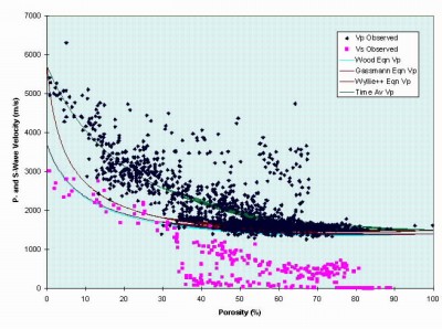 |
Figure 1. The distribution of sediments by their Porosity and P- and S-wave velocity values. Several separate populations are apparent. For P-wave velocities, the loose sediments with low velocities from 34% porosity and following the Gassmann function; consolidated sediments following the time-average relation; apparently cemented sediments with anomalously high velocities for the porosity. The S-wave populations have yet to be explained. |
5. Porosity Based on Mud Content of Loose Sediments
A compilation of many published analysis results (fig. 4) supports the empirical relationship:
mPor = 0.4 * mud + 43
for mud% > 7%. It appears to hold equally for terrigenous and carbonate sediments. Figure 2 illustrates the relationship for sediments of the Mississippi-Alabama-Florida (MAFLA) shelf.
 |
Figure 2. Empirical data supporting the Mud%-Porosity relation where mud fraction is >7%. The plotted data are a mix of terrigenous, carbonate, loose and consolidated samples, Mississippi-Alabama-Florida (MAFLA) shelf. |
6. Porosity Based on Average Grain size
Richardson and Briggs (1993) proposed a relationship between porosity and average grain size (AvGrsz, phi units) based on their measurements of muddy and sandy sediments. The relation is inverted for the onCALCULATION, and is applied only in the range AvGrsz > 0 phi:
Por = 26.92 + 5.92 * AvGrsz
The form is less accurate than methods where the percent of mud is known, and is not used in those cases.
7. Coarse Fraction and the P-wave Velocity
Related to the porosity-mud fraction function is another between coarse fraction and Vp:
mVp = 0.0009 * SpG³ + -0.14 * SpG² + 8.56 * SpG + 1512.76
where SpG is the percent coarse fraction. This polynomial is a poor fit and further work is required.
8. Wood-Gassmann Equation for P-wave Velocity in Loose Sediments
This method of estimating Vp is applied to sediments with no evidence of consolidation. It depends on assumed values for some acoustic constants of the sediments: (a) the Bulk Moduli K for solid, fluid, frame (Ko1Sol, Ko1Flu and Ko1Fra 3.6E+10, 2E+09 and 4E+08, MKS units) and (b) the Rigidities for solids and frame (RigidSol, RigidFra 2.2E+07, 1E+07).
The sediment Bulk Modulus and Density are:
Ko1 = (1-fPor)/Ko1Sol + fPor/Ko1Flu
SedDens = (1-fPor)*DenSol + fPor*DensFlu .
And the p-wave velocity is calculated as:
Qgass=Ko1Flu*(Ko1Sol-Ko1Fra)
(fPor*(Ko1Sol-Ko1Flu))
Kgass=Ko1Sol*(Ko1Fra+Qgass)/(Ko1Sol-Qgass)
VPgass=√(Kgass+4/3*RigidFra )/SedDens)
Gassmann (1951). VPgass is output as the estimate of Vp.
The Wood-Gassmann relation is one of several that have been proposed between porosity and the acoustic velocities. As can be seen on figure 1, the relation has an associated population of data ranging only between 35 and 80% porosity. In the dbSEABED onCALCULATION it is applied only where porosity is known and >35%, and where there is no indication of consolidation.
9. Roughness from Grain Protrusion for Gravels and Coarser Sediments
Kirchner and others (1990) offer a method for the calculation of grain protrusion (PnKir) above a sediment surface:
EnKir=0.5*(DnKir-D50Kir+(DnKir+D50Kir)*cos(F100nKir))
PnKir=EnKir+pi*D50Kir/12
where D50Kir and DnKir are the median and nth percentile grain sizes, and F100nKir is the Friction angle with a test grain of the 100-nth grain size percentile. In onCALCULATION the estimation is done only using the central and the coarsest grain sizes (CSESTsz; either PRS or EXT) for D50Kir and DnKir. PnKir is output as an estimate of roughness.
10. Roughness Metric from Outsized Clasts
This metric was employed as an early measure of seabed roughness; it is based on an idealized arrangement of the sediment clasts and particles. The coarsest grain size is logged from previous processing of grain size analysis and descriptive data inputs or is estimated from the average plus 2 times the SD (sorting) where both are known. The vertical roughness is estimated as half the clast size (D) with allowance for natural oblateness:
dZ=0.5 * D * CSF
where CSF is the Corey Shape Factor to account for non-sphereicity. (In naturally worn materials CSF is about 0.7; for example, Jimenez and Madsen 2003.) The spacing of the clast grain size is assessed as half the repeat distance implied by the fractional linear abundance PL of the outsized clast with size D. Linear abundance is related to areal and volume (most common) abundances PA and PV as: PL=PA1/2, PL=PV1/3 . The clast protrusion and half-spacing are output as the vertical and horizontal roughness scales.
11. Critical Shear Stress
If the material shows evidence of consolidation, then the Critical Shear Stress (CSS, N/m²) is set equal to the reported Shear Strength (kPa). Whitehouse and others (2000, p. 27) discuss the relationship, which is interim in the onCALCULATION.
For loose sediments, the functions related to grain size (AvGRZ) were investigated on the basis of data from many studies (fig. 3). This work was done in conjunction with IOW in Germany. The conclusions were (i) with fine-grained loose sediments where density or porosity are known, use the relationship of Mitchener and others (1996, in Whitehouse and others (2000)); (ii) else for those sediments use a generalized value of 0.5 N/m²; (iii) for loose coarse grained sediments use a log-linear relationship as shown in figure 3, log10(CSS)=log10[1.04-AvGRZ*0.6].
Bioturbation and bioconsolidation were not recognized in the estimation process for fine sediments, though they can be important (see Black and others (2002)). A correction of minor importance compared to the overall uncertainties is applied in the onCALCULATION.
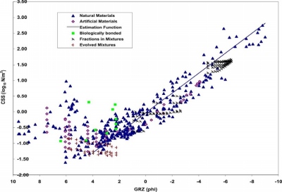 |
Figure 3. A compilation of Critical Shear Stress results by sediment grain size over the gravel to clay range. Over 24 references were used referring to marine and river sediments, field and laboratory experiments, on unaltered and manipulated natural sediments. |
|