Abstract: The 1994 Northridge, California, earthquake is the first earthquake for which we have all of the data sets needed to conduct a rigorous regional analysis of seismic slope instability. These data sets include (1) a comprehensive inventory of triggered landslides, (2) about 200 strong-motion records of the mainshock, (3) 1:24,000-scale geologic mapping of the region, (4) extensive data on engineering properties of geologic units, and (5) high-resolution digital elevation models of the topography. All of these data sets have been digitized and rasterized at 10-m grid spacing in the ARC/INFO GIS platform. Combining these data sets in a dynamic model based on Newmark's permanent-deformation (sliding-block) analysis yields estimates of coseismic landslide displacement in each grid cell from the Northridge earthquake. The modeled displacements are then compared with the digital inventory of landslides triggered by the Northridge earthquake to construct a probability curve relating predicted displacement to probability of failure. This probability function can be applied to predict and map the spatial variability in failure probability in any ground-shaking conditions of interest. We anticipate that this mapping procedure will be used to construct seismic landslide hazard maps that will assist in emergency preparedness planning and in making rational decisions regarding development and construction in areas susceptible to seismic slope failure.
Landslides are one of the most damaging collateral hazards associated with earthquakes. In fact, damage from triggered landslides and other ground failures has sometimes exceeded damage directly related to strong shaking and fault rupture. Seismically triggered landslides damage and destroy homes and other structures, block roads, sever pipelines and other utility lifelines, and block stream drainages. Predicting where and in what shaking conditions earthquakes are likely to trigger landslides is a key element in regional seismic hazard assessment.
Factors contributing to slope failure at a specific site are generally complex and difficult to assess with confidence; therefore, regional analysis of a large group of landslides triggered in a well-documented earthquake is useful in estimating general conditions related to failure. The 1994 Northridge, California, earthquake (M 6.7) presents the ideal case for such an analysis because all of the data sets required for detailed regional analysis of slope failures are available. We present here a method to map the spatial distribution of probabilities of seismic slope failure in any set of shaking conditions of interest. The method is calibrated using data from the 1994 Northridge earthquake, and it's application is demonstrated in the Oat Mountain 7 1/2´ quadrangle, on the northern edge of San Fernando Valley near Los Angeles, California.
We model the dynamic performance of slopes using the permanent-displacement analysis developed by Newmark (1965). Wilson and Keefer (1983) showed that using Newmark's method to model the dynamic behavior of landslides on natural slopes yields reasonable and useful results. Wieczorek and others (1985) subsequently produced an experimental map showing seismic landslide susceptibility in San Mateo County, California, using classification criteria based on Newmark's method. Wilson and Keefer (1985) also used Newmark's method as a basis for a broad regional assessment of seismic slope stability in the Los Angeles, California, area.
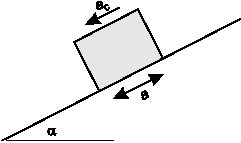
Newmark's method models a landslide as a rigid block that slides on an inclined plane (fig. 1). The block has a known critical (or yield) acceleration, ac, which is simply the threshold base acceleration required to overcome shear resistance and initiate sliding. The analysis calculates the cumulative permanent displacement of the block relative to its base as it is subjected to the effects of an earthquake acceleration-time history.
In the analysis, an acceleration-time history of interest is selected, and the critical acceleration of the slope to be modeled is superimposed (fig. 2A). Accelerations below this level cause no permanent displacement of the block. Those portions of the record that exceed the critical acceleration are integrated once to obtain the velocity profile of the block (fig. 2B); a second integration is performed to obtain the cumulative displacement history of the block (fig. 2C). The user then judges the significance of the displacement. Newmark's method is based on a fairly simple model of rigid-body displacement, and thus it does not necessarily precisely predict measured landslide displacements in the field. Rather, Newmark displacement is a useful index of how a slope is likely to perform during seismic shaking.
Newmark (1965) showed that the critical acceleration of a potential landslide block is a simple function of the static factor of safety and the landslide geometry, expressed as
![]()
where ac is the critical acceleration in terms of g, the acceleration of Earth's
gravity; FS is the static factor of safety; and![]() is the angle from the horizontal that the
center of mass of the potential landslide block first moves, which can generally be approximated as the slope angle.
Thus, conducting a Newmark analysis requires knowing the static factor of safety and the slope angle and selecting
an earthquake strong-motion record.
is the angle from the horizontal that the
center of mass of the potential landslide block first moves, which can generally be approximated as the slope angle.
Thus, conducting a Newmark analysis requires knowing the static factor of safety and the slope angle and selecting
an earthquake strong-motion record.
We developed and calibrated the methodology in the Oat Mountain 7 1/2´ quadrangle, which includes parts of the northern San Fernando Valley and Santa Susana Mountains (fig. 3). This quadrangle lies just a few kilometers north of the Northridge earthquake epicenter and contains dense concentrations of triggered landslides (Harp and Jibson, 1995, 1996). Topography ranges from flat areas in the San Fernando Valley to nearly vertical slopes in the Santa Susana Mountains. Predominant geologic units in the quadrangle include uncemented to weakly cemented late Tertiary clastic sediments and well-cemented Cretaceous sandstone.
The Northridge earthquake is the first earthquake for which we have all of the data sets needed to conduct a detailed regional analysis of factors related to triggered landsliding. These data sets include (1) a comprehensive inventory of triggered landslides (Harp and Jibson, 1995, 1996), (2) about 200 strong-motion records of the mainshock recorded throughout the region of landsliding, (3) detailed (1:24,000-scale) geologic mapping of the region, (4) extensive data on engineering properties of geologic units, and (5) high-resolution digital elevation models of the topography. All of these data sets have been digitized and rasterized at 10-m grid spacing in the ARC/INFO GIS platform. Combining these data sets in a dynamic model based on Newmark's permanent-deformation (sliding-block) analysis yields estimates of coseismic landslide displacement in each grid cell from the Northridge earthquake. The modeled displacements are then compared with the digital inventory of landslides triggered by the Northridge earthquake to construct a probability curve relating predicted displacement to probability of failure. Once calibrated with Northridge data, the probability function can be applied to predict the spatial variability of failure probability in any ground-shaking scenario of interest. Because the resulting hazard maps will be digital, they can be updated and revised with additional data that become available, and custom maps that model any ground-shaking conditions of interest can be produced when needed.
Figure 4 is a flowchart showing the sequential steps involved in the hazard-mapping procedure. Data layers consist of 10-m raster grids of the entire quadrangle. The sequence is relatively straightforward:
1. Compute the static factor of safety (ratio of resisting to driving forces).
A. Using compiled shear-strength data, assign representative shear strengths to each unit on the geologic map, which yields friction
and cohesion (c´) grids.
B. Construct a slope map from the digital elevation model (DEM).
C. Combine shear-strength and slope data in a factor-of-safety equation to estimate static factors of safety in each grid cell.
2. Compute the critical acceleration by combining the factor-of-safety grid with the slope grid to yield the critical-acceleration grid, which represents seismic landslide susceptibility.
3. Estimate Newmark displacements from the Northridge earthquake using an empirical regression equation to combine the critical- acceleration grid with the grid containingshaking-intensity values from the Northridge earthquake.
4. Construct a curve to estimate probability of slope failure as a function of Newmark displacement.
A. Compare the map of landslides triggered by the Northridge earthquake to the Newmark-displacement grid.
B. For sequential intervals of Newmark displacement, compute the proportion of cells containing landslides.
C. Plot the proportion of failed slopes in each interval as a function of Newmark displacement, and fit a regression curve.
5. Generate maps showing probability of seismic slope failure in any shaking scenario of interest.
A. Estimate Newmark displacements by combining a ground-shaking grid of interest with the critical acceleration grid, as in step 3.
B. Estimate probabilities of failure using the calibrated regression curve from step 4.
In the sections that follow, each of the steps outlined above is discussed in detail.
The dynamic stability of a slope, in the context of Newmark's method, is related to its static stability (see eq. 1); therefore, the static factor of safety for each grid cell must be determined. For purposes of regional analysis, we use a relatively simple limit-equilibrium model of an infinite slope in material having both frictional and cohesive strength. The factor of safety (FS) in these conditions is given by:
where ![]() is the effective friction angle,
c´ is the effective cohesion,
is the effective friction angle,
c´ is the effective cohesion,![]() is the
slope angle,
is the
slope angle,![]() is
the material unit weight,
is
the material unit weight, ![]() is
the unit weight of water, t is the slope-normal thickness of the failure
slab, and m is the proportion
of the slab thickness that is saturated. The equation is written so that the
first term on the right side accounts for the cohesive component of the strength,
the second term accounts for the frictional component, and the third
term accounts for the reduction in frictional strength due to pore pressure.
In the conditions modeled for this calibration, no pore-water pressure is included
(m=0) because almost all of the failures in the Northridge
earthquake occurred in dry conditions; thus, the third term drops from the equation.
For simplicity, the product
is
the unit weight of water, t is the slope-normal thickness of the failure
slab, and m is the proportion
of the slab thickness that is saturated. The equation is written so that the
first term on the right side accounts for the cohesive component of the strength,
the second term accounts for the frictional component, and the third
term accounts for the reduction in frictional strength due to pore pressure.
In the conditions modeled for this calibration, no pore-water pressure is included
(m=0) because almost all of the failures in the Northridge
earthquake occurred in dry conditions; thus, the third term drops from the equation.
For simplicity, the product![]() is taken to be 38.3 kPa (800 lbs/ft2), which reflects a typical unit
weight of 15.7 kN/m3
(100 lbs/ft3) and slab thickness of 2.4 m (8 ft), representative of
typical Northridge failures. The factor of safety, then, is calculated by inserting
values from friction, cohesion, and slope-angle grids into equation 2.
is taken to be 38.3 kPa (800 lbs/ft2), which reflects a typical unit
weight of 15.7 kN/m3
(100 lbs/ft3) and slab thickness of 2.4 m (8 ft), representative of
typical Northridge failures. The factor of safety, then, is calculated by inserting
values from friction, cohesion, and slope-angle grids into equation 2.
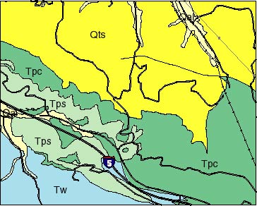
Geologic map: A digital geologic map forms the basis for assigning material properties throughout the area (fig. 5). We used the 1:24,000-scale digital geologic map of Yerkes and Campbell (1993, 1995). Representative values of the frictional and cohesive components of shear strength were assigned to each geologic unit.
Shear-strength data: Representative shear-strength values for geologic units were selected based on (1) compilation of numerous direct-shear test results from local consultants, (2) the judgment of several experienced geotechnical engineers and geologists in the region, and (3) the constraint that the computer slope model be statically stable.
We compiled results from hundreds of direct-shear tests on samples from a variety of geologic units in the quadrangle. In addition, we queried several experienced professionals from the local practicing and regulatory communities regarding representative shear-strength values for seismic conditions. There was broad agreement among these sources of information regarding the differences in strength between the various geologic units. In the initial iteration of the model, we assigned strengths near the middle of the ranges represented in our sources of information, and we adjusted strengths where needed to preserve the documented differences in strengths between units.
The Oat Mountain quadrangle has areas of very steep terrain, and the first factor-of-safety iteration yielded factors of safety less than 1 (indicating static instability) in some grid cells in steep areas. Our last constraint on assigning shear strengths to units, then, was that the model be statically stable, which simply means that no slopes be moving before the earthquake shaking occurs. We incrementally increased strengths of units having statically unstable cells, and then adjusted strengths of other units to preserve the documented strength differences between units. We did this iteratively until all slopes less than 60° were statically stable. A very small number (roughly a few dozen out of more than 1 million) of slopes steeper than 60° remained unstable even at rather high strengths; therefore, we assigned a minimal factor of safety of 1.01, barely above equilibrium, to these slopes to avoid increasing the strengths beyond realistic levels.
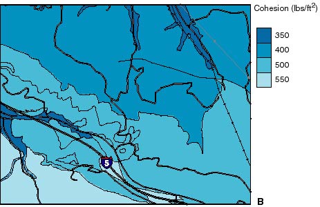
Table 1 shows strengths assigned to geologic units. These strengths clearly should be considered peak strengths and represent the higher end of the range of probable strength variation within a given unit because they are strengths required to maintain static stability in the very steepest of slopes within that unit. As will become clear later in the analysis, the absolute value of the assigned strength is less important than the relative strength differences between units, and those differences are reasonably well constrained in a regional sense. Figure 6 shows the (A) friction and (B) cohesion values assigned to the geologic units in a part of the area.
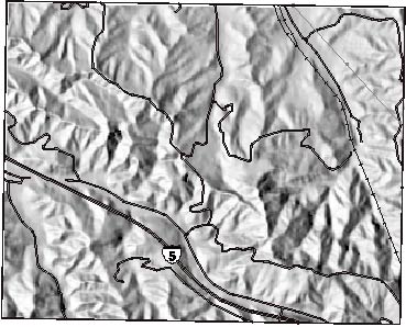
Digital elevation model: The 10-m digital elevation model (DEM) was produced by high-resolution scanning of the original USGS contour plates of the 1:24,000-scale Oat Mountain 7 1/2´ quadrangle (fig. 7). We selected a 10-m scanning resolution to preserve the subtle topographic features in which many landslides occur; too many topographic irregularities are lost in the more commonly used 30-m DEMs. It must be remembered, however, that the DEM is simply a digital representation of the original contour map: higher resolution scans produce DEMs that more faithfully reflect the published contour map, but they do not improve on any limitation that map may have.
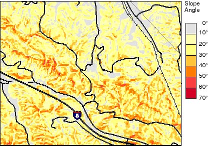
Slope Map: The slope map (fig. 8) was produced by applying a simple algorithm to the DEM that compares the elevations of adjacent cells and computes the maximum slope. The slope map tends to underestimate some of the steepest slopes (steeper than about 60°) primarily because such slopes are not well represented on the original contour map.
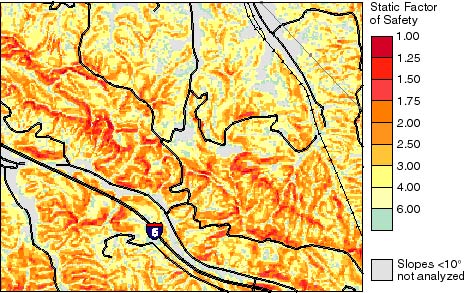
Factor-of-Safety Map: Figure 9 shows a part of the factor-of-safety map resulting from combining these data layers in equation 2. Factors of safety range from just greater than 1.0, for steep slopes in weak material, to more than 8 for flatter slopes in strong material.
As indicated above, Newmark (1965) showed that the critical acceleration of a slope is a simple function of its static factor of safety and the slope angle (see eq. 1). Therefore, producing a critical-acceleration grid (pl. 1) is a simple matter of using equation 1 to combine the slope angle with the calculated factors of safety.
Within the context of the Newmark-displacement analysis, critical (or yield) acceleration uniquely describes the dynamic stability of a slope. For a given shaking level, any two slopes that have the same critical acceleration will yield the same Newmark displacement, regardless of how those slopes might differ in geometry or material properties. The critical-acceleration map portrays a measure of intrinsic slope properties independent of any ground-shaking scenario; thus, it is a map of seismic landslide susceptibility.
A rigorous Newmark analysis is conducted by double integrating the parts of a specific strong-motion record that exceed the critical acceleration. For a regional hazard analysis, conducting a rigorous Newmark analysis in each 10-m-grid cell is both impractical and inappropriate. For each grid cell, a unique strong-motion record would have to be procured or artificially produced, and such a record would model only one of a broad range of possible ground-shaking levels.
To facilitate using Newmark's method in regional analysis, Jibson (1993) developed a simplified Newmark method wherein an empirical regression equation is used to estimate Newmark displacement as a function of shaking intensity and critical acceleration. We slightly modified the functional form of that equation to make the critical acceleration term logarithmic, and we used a much larger group of strong-motion records--280 recording stations in 13 earthquakes (table 2) -to develop a new regression equation. (With this larger data set, a logarithmic critical-acceleration term yielded a much better fit than a linear term.) We analyzed both of the horizontal components of acceleration from 275 of the recordings and a single component from the remaining 5, which yielded 555 single-component records. For each record, we determined the Arias (1970) intensity, a single numerical measure of the shaking intensity of the record calculated by integrating the squared acceleration values (Jibson, 1993). We then conducted a Newmark analysis for several values of critical acceleration, ranging from 0.02 g to 0.40g. The resulting Newmark displacements were then regressed on two predictor variables: critical acceleration and Arias intensity. The resulting regression equation is
![]()
where Dn is Newmark displacement in centimeters, Ia is Arias intensity in meters per second, and ac is critical acceleration in g's. The regression equation is well constrained (R2=83 percent) with a very high level of statistical significance, the model standard deviation is 0.375. Thus, Newmark displacement, an index of seismic slope performance, can be estimated as a function of critical acceleration (dynamic slope stability) and Arias intensity (ground-shaking intensity).
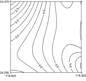
The distribution of landslides triggered by the Northridge earthquake was used to calibrate the modeling procedure; therefore, we produced a ground-shaking grid from the Northridge earthquake. For each of 189 strong-motion recordings of the mainshock, we plotted the average Arias intensity from the two horizontal components. We then used a simple kriging algorithm to interpolate values across a regularly spaced grid (fig. 10).
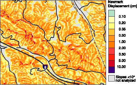
Newmark displacements from the Northridge earthquake were estimated in each grid cell of the Oat Mountain quadrangle (fig. 11) by using equation 3 to combine corresponding grid values of critical acceleration and Arias intensity. Predicted displacements range from 0 to 3038 cm.
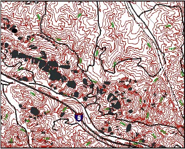
Predicted Newmark displacements do not necessarily correspond directly to measurable slope movements in the field; rather, modeled displacements provide an index to correlate with field performance. For the Newmark method to be useful in a predictive sense, modeled displacements must be quantitatively correlated with field performance. In short, do larger predicted displacements relate to greater incidence of slope failure? Comparison of the predicted Newmark displacements (fig. 11) with the actual inventory of landslides triggered by the Northridge earthquake (fig. 12) allows us to answer this question.
The Newmark-displacement grid cells were grouped into bins, such that all cells having displacements between 0 and 1 cm were in the first bin; those having 1 to 2 cm of displacement were in the second bin, and so on. For displacements greater than about 10 cm, the number of cells in 1-cm bins became very small; therefore, broader ranges of displacement were grouped together to provide a statistically significant number of cells in each bin. For each bin, the proportion of the cells that were in landslide source areas was calculated. Landslide source areas were defined to include those grid cells having elevations above the median elevation for each landslide, so that the upper half of each landslide was considered a source area.
Figure 13 shows, for each bin, the proportion of cells occupied by landslide source areas plotted as a function of Newmark displacement. The data clearly demonstrate the utility of Newmark's method to predict the spatial density of seismically triggered landslides: the proportion of landslide cells within each displacement bin increases monotonically with increasing Newmark displacement. The proportion of landslide cells increases rapidly in the first few centimeters (bins) of Newmark displacement and then levels off abruptly in the 10- to 15- cm range at a proportion of about 27 percent. This relation is critical in a predictive sense because the proportion of landslide cells in a given displacement bin is a direct estimate of the probability or percent chance that any cell in that displacement range will be occupied by a landslide source.
We chose to fit the data in figure 13 with a Weibull (1939) curve, which was initially developed to model the failure of rock samples (Jaeger and Cook, 1969). The functional form produces an S-shaped curve that is apparent in the data:
![]()
where P(f) is the proportion of landslide cells, m is the maximum proportion of landslide cells indicated by the data, Dn is the Newmark displacement in centimeters, and a and b are the regression constants to be determined. The expression inside the brackets takes the form of the original Weibull equation, which yields values ranging from 0 to 1; the m outside the brackets simply scales this range to reflect the range represented by the data. The regression curve based on the Northridge data is
![]()
The curve fits the data extremely well (R2=95.9 percent), and prediction of the proportion of landslide cells (P(f)) can be used to directly estimate probability of slope failure as a function of Newmark displacement. Once calibrated, the curve and corresponding equation can be used in any set of ground-shaking conditions to predict probability of slope failure as a function of predicted Newmark displacement.
Figure 13 and equation 5 provide the necessary linkage between the displacements estimated from the Newmark model and probabilities of landslide occurrence in the field. The curve thus forms the basis for producing seismic landslide hazard maps, which portray spatial variation in slope-failure probability in a specified set of ground-shaking conditions. Plate 2 shows such a map for the Oat Mountain quadrangle for the ground-shaking conditions experienced in the Northridge earthquake. Northridge-triggered landslides also are shown to demonstrate how well the mapping procedure captured what actually happened. The fit appears to be very good: most of the triggered landslides lie in the higher probability (warmer colored) areas, and most such areas contain landslides.
Constructing a hazard (probability) map for other ground-shaking scenarios is equally straightforward, provided the ground shaking can be reasonably modeled. Such a procedure would involve the following:
Nearly all of the variability in failure probability (fig. 13) occurs in the first few centimeters of displacement; for displacements greater than about 15 cm, no measurable increase in failure probability is predicted. This is perhaps attributable to the fact that the vast majority of landslides in the database were shallow, disrupted rock falls and rock slides in fairly brittle, weakly cemented sediments that fail at relatively small displacements. The shape of the curve strongly suggests brittle failure: most of what is going to fail does so within a narrow and relatively low range of displacements.
A maximum proportion of failed slopes of 25-30 percent is reasonable in light of our experience in documenting triggered landslides in numerous worldwide earthquakes. We have rarely seen more than 25 percent of slope areas fail, even on the most susceptible slopes in epicentral areas. In terms of slope area, a failure rate of 25-30 percent is catastrophic.
The overwhelming majority of landslides triggered by the Northridge earthquake were relatively shallow, disrupted slides and falls in rock and debris (Harp and Jibson, 1995, 1996). Therefore, any model calibrated from these data is useful primarily for predicting the spatial distribution of these types of landslides. The small number of deeper, more coherent slides triggered by the Northridge earthquake did not produce a statistically significant sample that could meaningfully contribute to the model. Thus, the distribution of deep, coherent landslides will probably be less accurately predicted using this calibration (eq. 5) than will the distribution of shallow, disrupted slides. Indeed, in most worldwide earthquakes, disrupted landslides are by far the predominant landslide type (Keefer, 1984), and so landslide distributions predicted using this method and calibration should relate well to typical distributions of triggered landslides.
As discussed previously, shear strengths used in the model reflect peak strengths in order to render the model statically stable. Relative strengths between units, however, are much more important than the absolute strength values, and relative strengths are reasonably well constrained. The calibration (eq. 5) is based on the strengths selected, and that calibration is only rigorously valid for models using the strengths in this paper. Using reduced strengths, either to represent residual-strength conditions or to simply take a more conservative approach, will not yield accurate results using equation 5. To appropriately use different strengths, the model would have to be recalibrated, which would presumably yield an equation similar to equation 5 but having different coefficients and exponents.
Shear strength typically has large spatial variability in nature even within geologic units, and assigning representative shear strengths to entire units is fraught with uncertainty. The modeling procedure, however, is heavily slope-driven. The effects of slope angle on the model output far outweigh the effects of modest differences in material strength; therefore, highly accurate characterizations of strength are not deemed essential. For example, the slight differences in strength between the different late Tertiary, weakly cemented units (table 1) are virtually insignificant in terms of the model output. The much larger strength difference between these units and the well-cemented Chatsworth Formation, however, is very significant. Thus, assignment of strengths is primarily important in differentiating units having large strength differences.
The probability equation can be applied using any set of ground-shaking conditions of interest. The equation was calibrated using data from southern California, however, and applying it to regions that have greatly differing climates, rock types, vegetation, or topography increases the uncertainty of the results. Recalibration for use in different regions is desirable, but data sets for such calibration are generally lacking. Therefore, if this method is applied in other regions using equation 5, greater uncertainty in the output must be assumed. Values of a, b, and m (eqs. 4, 5) could vary in other regions if the strengths of geologic materials, topography, vegetation, or soil moisture conditions were significantly different from those in southern California. In regions where the predominant failure type is different, the shape of the curve (fig. 13) would probably be somewhat different as well. For example, if slumps and block slides in more compliant (less brittle) materials were predominant, the curve would likely be less steep and could flatten out at a larger maximum displacement value.
Maps produced using the method documented in this paper can be useful in emergency preparedness planning, lifeline siting and maintenance, critical-facility siting, long-term land-use planning, and a variety of other applications. Maps using this method, however, do not supersede published regulatory maps, such as the seismic hazard zonation maps issued by the California Division of Mines and Geology.
Analysis of data from the Northridge earthquake allows quantitative physical modeling of conditions leading to coseismic slope failure. If data sets describing the topography, geology, shear strength, and seismic shaking of an area or region can be procured, the procedure described in this paper can be used to produce hazard maps showing the spatial distribution of slope-failure probability. Within the limitations discussed, such maps can find useful application in regional seismic hazard and risk assessment.
Even considering all of the caveats and limitations discussed, this analytical mapping procedure provides a simple, systematic, physically based method to estimate seismic slope-failure probability. The linkage of Newmark displacement to a discrete failure probability is an enormously useful tool that will give Newmark's well-established method of analysis far more practical utility.
The Los Angeles County Department of Public Works and Leighton and Associates provided extensive data on material shear strengths. David Perkins and William Savage of the U.S. Geological Survey provided helpful insights into the statistical modeling of the failure data. David Keefer of the U.S. Geological Survey reviewed the manuscript. Graphic design and layout prepared by Eleanor M. Omdahl and Pamela S. Detra.
Arias, A., 1970, A measure of earthquake intensity, in Hansen, R.J., ed., Seismic design for nuclear power plants: Cambridge, Massachusetts Institute of Technology Press, p. 438-483.
Harp, E.L., and Jibson, R.W., 1995, Inventory of landslides triggered by the 1994 Northridge, California earthquake: U.S. Geological Survey Open-File Report 95-213, 17 p., 2 plates.
Harp, E.L., and Jibson, R.W., 1996, Landslides triggered by the 1994 Northridge, California earthquake: Bulletin of the Seismological Society of America, v. 86, no. 1B, p. S319-S332.
Jaeger, J.C., and Cook, N.G.W., 1969, Fundamentals of Rock Mechanics: London, Methuen and Company, 513 p.
Jibson, R.W., 1993, Predicting earthquake-induced landslide displacements using Newmark's sliding block analysis: Transportation Research Record, no. 1411, p. 9-17.
Keefer, D.K., 1984, Landslides caused by earthquakes: Geological Society of America Bulletin, v. 95, p. 406-421.
Newmark, N.M., 1965, Effects of earthquakes on dams and embankments: Geotechnique, v. 15, no. 2, p. 139-160.
Weibull, W., 1939, A statistical theory of the strength of materials: Ingenioersvetenskaps-akademien Stockholm Handlingar, no. 151.
Wieczorek, G.F., Wilson, R.C., and Harp, E.L., 1985, Map showing slope stability during earthquakes in San Mateo County California: U.S. Geological Survey Miscellaneous Investigations Map I-1257-E, scale 1:62,500.
Wilson, R.C., and Keefer, D.K., 1983, Dynamic analysis of a slope failure from the 6 August 1979 Coyote Lake, California, earthquake: Bulletin of the Seismological Society of America, v. 73, p. 863-877.
Wilson, R.C., and Keefer, D.K., 1985, Predicting areal limits of earthquake-induced landsliding, in Ziony, J.I., ed., Evaluating Earthquake Hazards in the Los Angeles Region-An Earth-Science Perspective: U.S. Geological Survey Professional Paper 1360, p. 316-345.
Wilson, R.C., 1993, Relation of Arias intensity to magnitude and distance in California: U.S. Geological Survey Open-File Report 93-556, 42 p.
Yerkes, R.F., and Campbell, R.H., 1993, Preliminary geologic map of the Oat Mountain 7 1/2´ quadrangle, southern California: U.S. Geological Survey Open-File Report 93-525, 13 p.
Yerkes, R.F. and Campbell, R.H., 1995, Preliminary geologic map of the Oat Mountain 7 1/2´ quadrangle, southern California-A digital database: U.S. Geological Survey Open-File Report 95-89.
LIST OF FIGURES, TABLES, AND PLATES
Figure 1. Sliding-block model used for Newmark analysis. The potential landslide is modeled as a block resting on a plane inclined at an angle (
) from the horizontal. The block has a known critical (yield) acceleration (ac), the base acceleration required to overcome shear resistance and initiate sliding with respect to the base. The block is subjected to a base acceleration (a) representing the earthquake shaking.
Figure 2. Demonstration of the Newmark-analysis algorithm (adapted from Wilson and Keefer, 1983). A, Earthquake acceleration-time history with critical acceleration (horizontal dashed line) of 0.20 g superimposed. B, Velocity of landslide block versus time. C, Displacement of landslide block versus time.
Figure 3. Location of Oat Mountain 7 1/2° quadrangle, California. Bold line is limit of landslides triggered by Northridge earthquake; shaded area shows zone of greatest landslide concentration; star is Northridge epicenter. Inset box shows sample area referred to in subsequent figures.
Figure 4. Flow chart showing steps involved in producing a seismic landslide hazard map.
Figure 5. Geologic map of part of the Oat Mountain quadrangle (location shown in fig. 3).
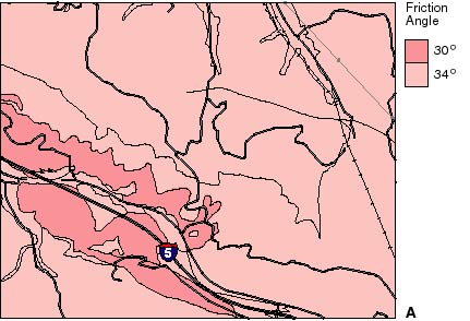
Figure 6. Map showing (A) frictional component and (B) cohesive component of shear strength (1lb/ft2 = 0.0479 KPa) assigned to geologic units in part of the Oat Mountain quadrangle (location shown in fig. 3).
Figure 7. Shaded-relief digital elevation model (DEM) of part of the Oat Mountain quadrangle (location shown in fig. 3).
Figure 8. Slope map derived from DEM of part of the Oat Mountain quadrangle (location shown in fig. 3).
Figure 9. Static factor-of-safety map of part of the Oat Mountain quadrangle (location shown in fig. 3).
Figure 10. Contours of Arias intensity (Ia) generated by the 1994 Northridge earthquake in the Oat Mountain quadrangle. Intensity values shown are the average of the two horizontal components.
Figure 11. Map showing predicted Newmark displacements in part of the Oat Mountain quadrangle (location shown in fig. 3).
Figure 12. Map showing landslides triggered by the Northridge earthquake (Harp and Jibson, 1995) in part of the Oat Mountain quadrangle (location shown in fig. 3).
Figure 13. Proportion of landslide cells as a function of Newmark displacement.
Table 1. Shear strengths assigned to geologic formations in the Oat Mountain Quadrangle.
Table 2. Sources of strong-motion records used to model Newmark displacement.
Plate 1. Oat Mountain quadrangle showing critical acceleration of a slope.
Plate 2. Oat Mountain quadrangle showing ground-shaking conditions experienced in the Northridge earthquake.
This report is preliminary and has not been reviewed for conformity with U.S. Geological Survey editorial standards or with the North American Stratigraphic Code. Any use of trade, product, or firm names is for descriptive purposes only and does not imply endorsement by the U.S. Government.

U.S. Department of the Interior | U.S. Geological Survey
URL: http://pubsdata.usgs.gov/pubs/of/1998/ofr-98-113/ofr98-113.html
Page Contact Information: GS Pubs Web Contact
Page Last Modified: Wednesday, 07-Dec-2016 16:46:43 EST