Open-File Report 99-7-B
Chapter 3
An interpretation of digital conductivity depth transform data from the 1997 Airborne ElectroMagnetic (AEM) survey, Fort Huachuca vicinity, Cochise County, Arizona
By Mark W. Bultman and Mark E.Gettings
Go to contentsThe upper resistivity minimum of the digital CDT vertical profiles may serve as a good approximation of the water table elevation in some regions of this study, it does not work well in all regions. Where the upper resistivity minimum correlates to the water table, it is unknown if it is due to the water table alone or to clay and silt facies in the basin fill. This methodology can be used to approximate the elevation of the water table in regions with no water wells. In the upper San Pedro basin, the actual water table elevation estimated from well water levels is more accurate.
The upper San Pedro basin is bounded on the west by a high angle fault near the edge of the basin. There is a bedrock high in the Sierra Vista area that extends to the east about 10 kilometers into the basin. South of the bedrock high the basin is complex, but seems to be shallower than north of the bedrock high. To the east of the basin bounding fault near the Huachuca Mountains and east of the Sierra Vista bedrock high, the basin remains deep until it approaches the Tombstone Hills. The relationship between the basin sediments and the bedrock in the Tombstone Hills area is complex and may be both stratigraphic and fault bounded.
The sediment fill in the basin contains many interfingered layers of clays and silts with coarser grained material. In general though, the thickness and amount of fine grained, low energy environment derived material is greater on the eastern edge of the basin. This zone thins towards the west. On the western edge of the basin, the dominant fill material is likely the gravel, sand, and unconsolidated material that is mapped at the surface.
note: This report is intended for viewing on a HTML version 2.0 or higher compatible browser. If you want to print this chapter, you may want to purchase the CD-ROM version of this publication which contains postscript files associated with each figure. The CD-ROM version is USGS Open-File Report 99-7-A and is for sale by calling (888) ASK-USGS.
Introduction
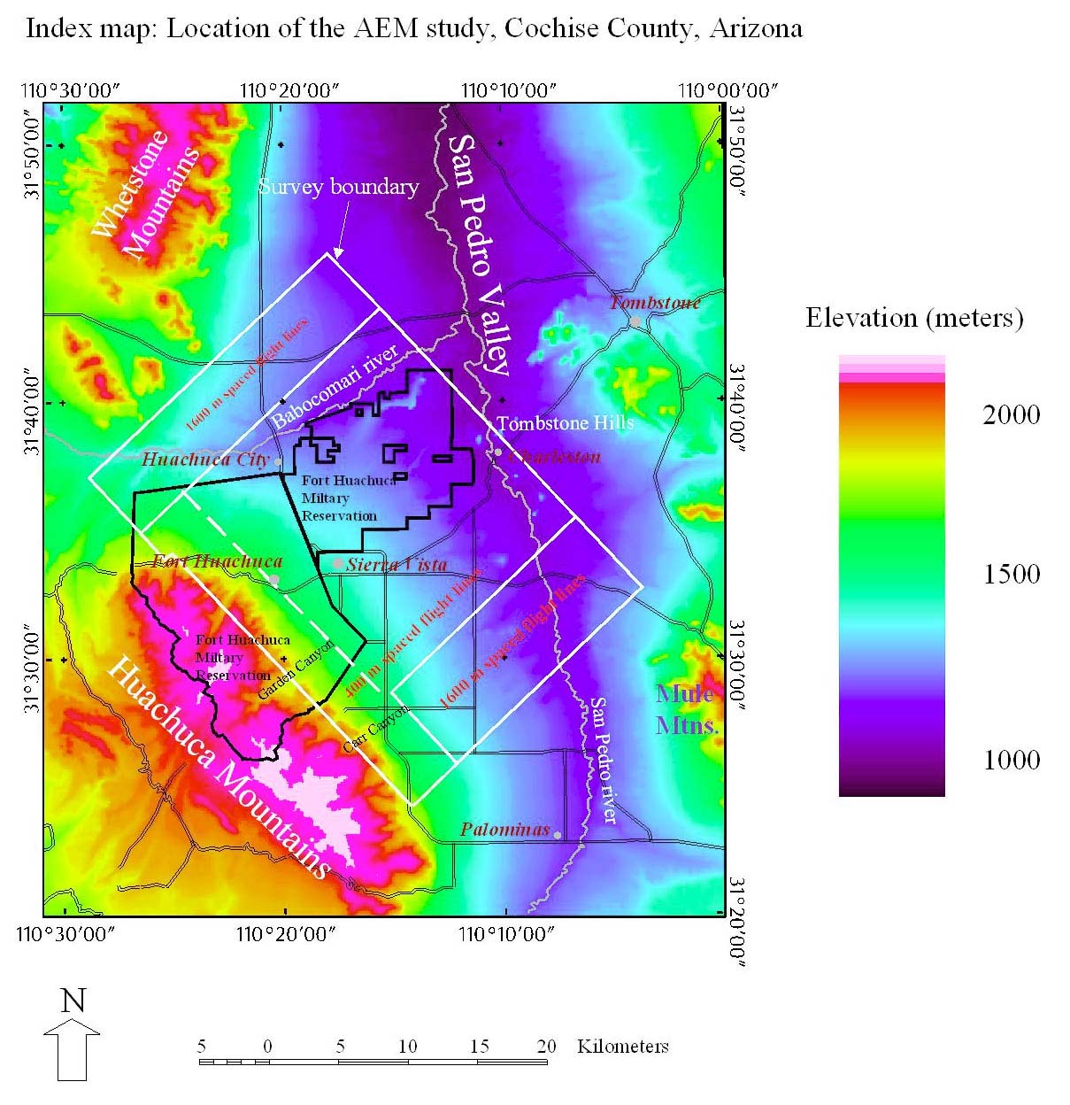
In March, 1997 an airborne time-domain electromagnetic (AEM) survey was flown over the Upper San Pedro Basin for the Environment and Natural Resources Division of the U.S. Army’s Garrison at Fort Huachuca, Arizona. The survey was designed to increase the understanding of the geometry of the basin, the composition of sediments in the basin, and to see what relationship, if any, can be made between the interpreted data from the survey and the water table in the basin. The survey itself is described in detail in Chapter 2 of this report.
One product of the AEM survey is a conductivity-vs-depth section derived by a mathematical calculation of the 120-channel airborne electromagnetic data acquired by the geophysical survey system. These calculations are referred to as conductivity depth transforms or CDTs. The mathematical technique used to obtain the CDTs is described by Wolfgram and Karlik (1995). While not technically a true inversion, the technique produces similar results as a true inversion based on the diffusion equation yet requires much less computation. The CDT data is delivered two ways, printed images for each CDT corresponding to each flight line and the digital data associated with each CDT. In addition, the raw digital data acquired during the survey is included. This includes the raw 120-channel airborne electromagnetic data as well as GPS, barometric altimeter, and radar altitude data. This chapter analyses the digital CDT data, and the terms digital CDT and CDT are both used to mean the same thing, the CDTs that are built from the digital CDT data.
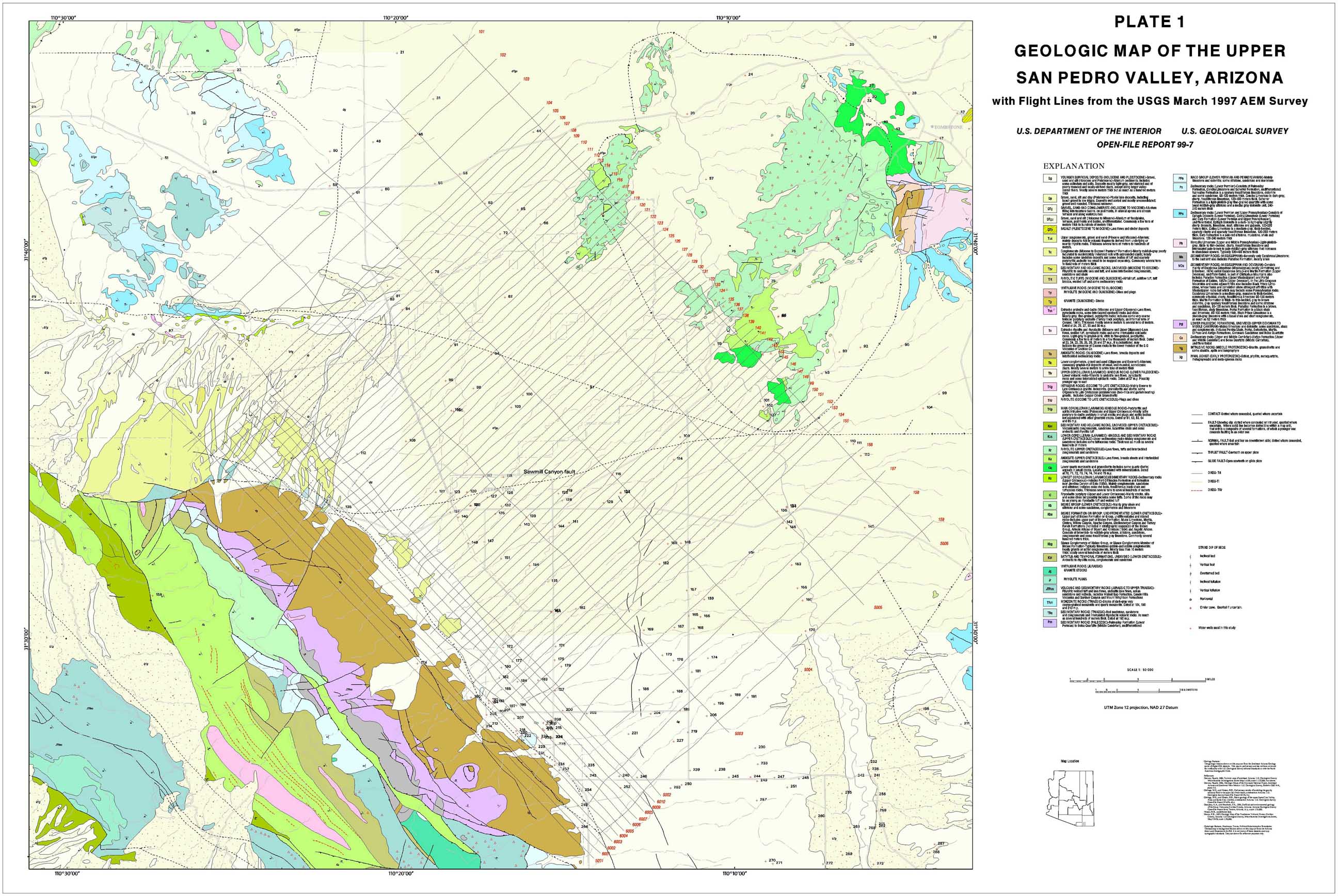
Plate 1 displays the flight lines which together comprise the AEM survey of the upper San Pedro basin. Due to the topography of the region, the direction of the flight lines for the southwest portion of the survey is perpendicular to the majority of the survey. While the aircraft may have flown along the flight line in either direction, the CDTs are organized so that their start points are all on one side of a set of parallel flight lines. The southwest-northeast striking CDTs (lines 101 through 159) all start near the southwest most point of the flight line. Lines 104 through 155 are spaced 400 meters apart, the rest are 1600 meters apart.
Go to plate 1 (5.3 MB compressed JPEG image)
The start points for the southeast-northwest striking flight lines are set near the southeast end of the line. The southeast-northwest striking flight lines are really two separate sets of lines. The lines 5001 through 5006 are tie lines that are used get some closely space data perpendicular to the majority of the flight lines and to check the integrity of the other survey lines. They are spaced at about 4.5 kilometers apart. The lines 6001 through 6010 are lines that are spaced at 400m but flown in between the first two tie lines, 5001 and 5002. The high elevation of the Huachuca foothills at the western margin of the survey mandated that the southwest-northeast striking flight lines end short of the intended coverage area, thus the lines 6001 through 6010 were flown to complete the survey.
The digital CDT data were prepared two ways for two purposes. The first method organized the data for a statistical analysis and is referred to as the location database. The second method built a three-dimensional data cube so that the data could be viewed with a volumetric viewer. This volumetric database is referred to as the data cube.
To build the location database, the data from each digital CDT was projected to its proper location using the CDT starting point, the rotation angle of the CDT (the CDT is essentially parallel to the flight line) and the distance between each data point on the CDT. The elevation of each point was based on the depth of investigation of the survey (1500m), the barometric elevation of the top of the survey (2200 meters), and the number of data points in a vertical section (128). So, at a given location, data points began at 711.72 meters elevation (the top of a data increment from 700 to 711.72 meters) and continued upward for 128 data increments to 2200 meters elevation. Points with no data were excluded from the database.
For the three-dimension data cube, the data were processed quite differently. The data from flight lines 101 through 159 were put together into one data cube, referred to as block 1. Between the 1600 meter spaced data, CDTs were built at a 400 meter spacing by a distance weighted average of the CDTs on either side. The data from flight lines 5001, 6001 through 6010, 5002 was put together in a second data cube referred to as block 2. These two data cubes (block 1 and block 2) were required to deal with the different directions of the flight lines in these areas. The remaining tie lines, 5003 through 5006, were not used in the volumetric data. The CDTs were processed for differences in the starting and ending points of each flight-line and for differences in the down flight-line distances between sample points. The processed data were then introduced into three-dimension visualization software that allows the resulting volume to be visualized from any perspective.
note: In this report conductivities and resistivities are both used, depending on the data we are dealing with. Well-logs are almost always reported as resistivity vs. depth, whereas most AEM systems report conductivities. For reasons of comparison with well logs, the CDTs used in this chapter were converted from conductivity values to resistivity values. Resistivity is simply the inverse of conductivity: resistivity = 1/conductivity . Resistivity is measured in ohm-meters. We have taken precautions throughout this report, in an attempt to avoid confusion, to relate the electrical values observed (or calculated in the case of the CDTs) to the lithology and porosity of the underlying rocks and unconsolidated sediments we are mapping.
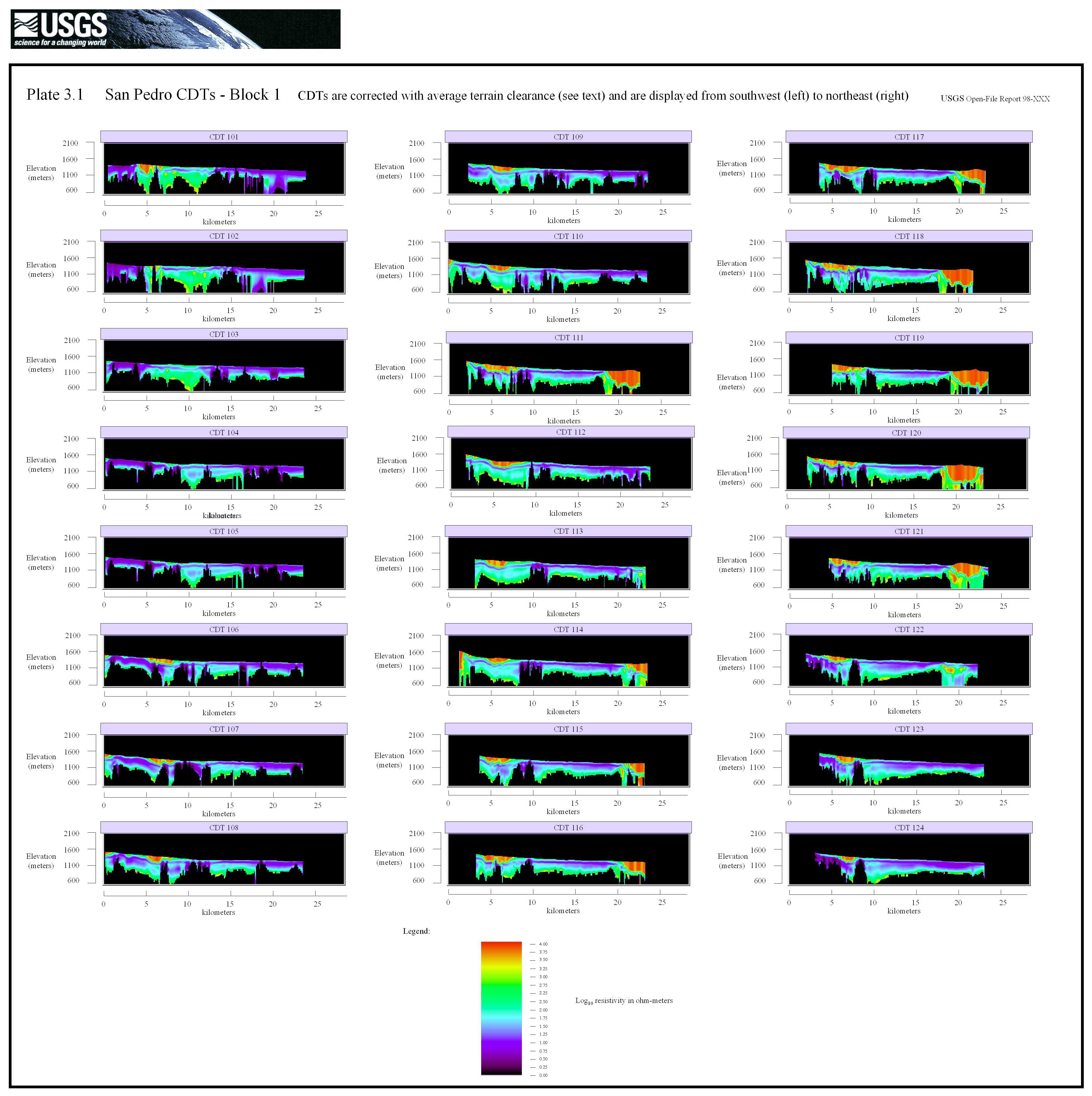
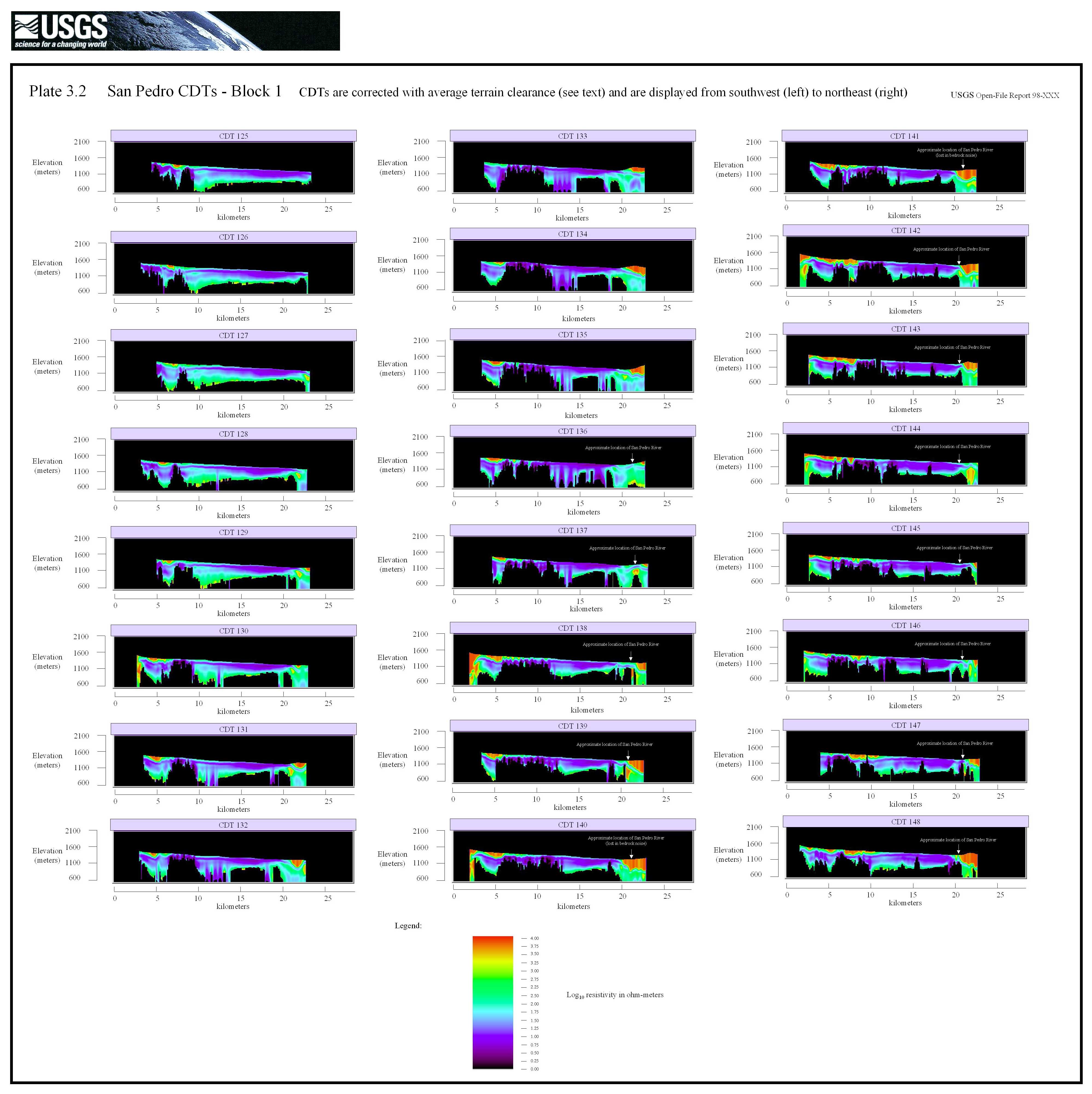
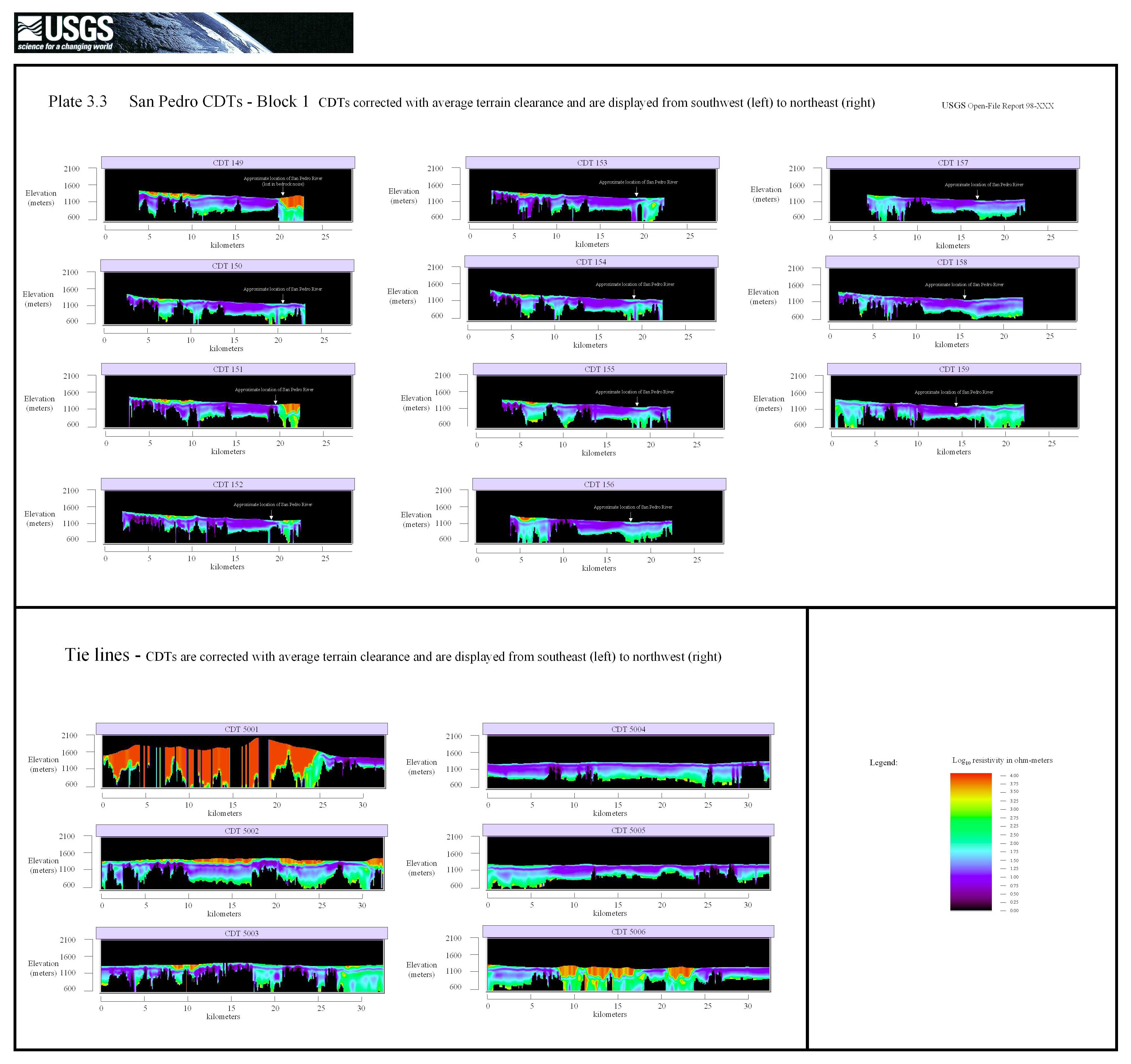
All digital CDT data has been plotted and is shown in plates 3.1 through 3.4. Plate 3.1 contains block 1 CDTs 101 through 124. Plate 3.2 contains block 1 CDTs 125 through 148. Plate 3.3 contains block 1 CDTs 149 through 159, as well as the tie line CDTs (5001 through 5006). Plate 3.4 contains Block 2 CDTs 5001, 6001 through 6010, and 5002. The top of the data in the original digital CDTs is supposed to represent the ground surface. Well into the analysis of the digital CDT data, we found that this was not the case. In fact, the top of the digital CDT data represents the elevation of the survey aircraft. The CDTs in figure 3.2 through 3.5 have had the average terrain clearance subtracted from the, so the top of the data represents the elevation of the survey aircraft minus 133.6 meters. This is a good approximation for the ground in the central portion of the basin, but a less than a good approximation in areas of steep topography. The elevation problem in the digital CDT data is discussed further in the next section.
Go to plate 3.1 (1.0 MB JPEG image)
Go to plate 3.2 (1.0 MB JPEG image)
Go to plate 3.3 (0.9 MB JPEG image)
Go to plate 3.4 (0.8 MB JPEG image)
To force a download instead of viewing, do the following:
Macintosh: hold the mouse button down for a moment to display a pop-up menu and select "Save this link as..." (Netscape Navigator) or "Download Link to Disk" (Internet Explorer) and navigate to where you want the file saved.
Windows machines: use the right mouse button to display a pop-up menu and select "Save Link As..." (Netscape Navigator) or "Save Target As..." (Internet Explorer) and navigate to where you want the file saved.
Problems with the digital CDT data
According to Geoterrex (Geoterrex-Dighem, 1997, appendix G), the digital CDTs are constructed using an algorithm that incorporates the barometric elevation and the radar altimeter to produce CDTs where the highest data point represent the topography of the ground surface. This correction is done, according to Geoterrex (Geoterrex-Dighem, 1997, appendix G), in order to deal with geometric problems that may be introduced into the CDTs in areas with a large relief. This way, dipping layers on the CDT are supposed to present the actual dip of a layer, not apparent dip due to the topography.
While analyzing vertical profiles of digital CDT data it was noted that the CDT data plotted well above where the ground surface should be. In an attempt to solve this problem, the exact location of the starting point of many CDTs were plotted on a topographic map and the elevation was obtained for each CDT starting point. The raw data point nearest each CDT starting point was found, and from this point, the barometric and GPS elevations as well as the radar altimeter values were read. When this data was all plotted (figure 3.1), the elevation of each CDT start point was found to be identical or nearly identical to the GPS elevation for the original data. Any differences can be attributed to the accuracy of the topographic map or the fact that the CDTs do not line up perfectly with the flight lines.
Figure 3.1:
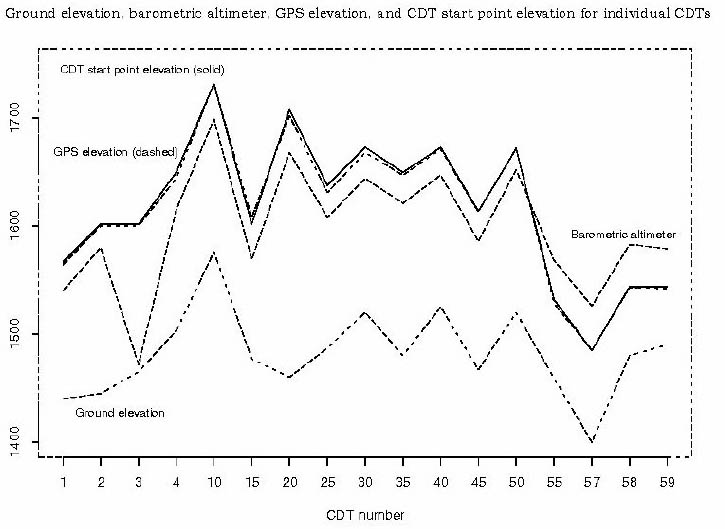
Figure 3.1 indicates that the CDTs must have been computed using the only the GPS elevation, the radar altimetry was not subtracted. This probably has two effects on the CDTs themselves, but without access to the algorithm that produced the CDTs, these are only estimates of the effects. First, since the algorithm that computes the CDTs thinks that the sensor is much closer to a conductive bodies than it really is, the conductivity attributed to a given signal may be underestimated. The signal that it sees is smaller due to the fact that the sensor is, in reality, farther away from the conductive medium. Second, geometric problems must be introduced. The algorithm calculates the conductivities directly below the location where the data was acquired. But in this case, it is being fed the elevation of the survey plane not the topography, and the survey plane can not perfectly drape the topography. In areas where the survey plane was forced to vary from its specified terrain clearance, the geometric relationships in the original CDT data may be somewhat distorted.
Because many of the analyses in this report are based on having the proper elevation of each data point in the CDTs, the digital CDT data used to build the location data base was corrected by subtracting the radar altimeter reading from the raw data point nearest each CDT point. Due to a lack of time, the data cube was corrected differently. The elevations in the data cube were corrected by subtracting the mean of the terrain clearance (133.67 meters). This means that the surface shown as the ground (the top of the data) in plates 3.1 through 3.4 actually represents the altitude of the plane minus the mean terrain clearance.
Analysis of digital CDT resistivity and its relationship to the water table in the upper San Pedro basin
Introduction
The CDTs contain resistivity-vs-depth information that was calculated over a point from data acquired during the AEM survey. Differences in resistivity can be interpreted as lithologic changes in the sedimentary column. We assume that sediments composed primarily of sands and gravels are more resistive than sediments composed primarily of silts and clays. Sediments that are saturated with water, or that contain some water content, are likely to have a lower resistivity than sediments that are dry. To test whether the calculated resistivities observed in the CDT data are affected by the water table, we will compare the shape and values of the CDT resistivity at locations where the depth to the water table is known.
Resistivity at the water table
The CDTs, as used in this analysis, display a theoretical resistivity at a given depth. By using a database of known water wells (Tatlow, 1998) and the digital CDT location data, its possible to look at resistivities near the water table in a statistical sense. In order to compare these resistivities, it is necessary to find the closest CDT point to a water well. Software was written for this purpose and the resulting data allows the mean and variance of the resistivity at the water table for each well to be calculated.
Several combinations of maximum distance from the water well were tried including 100, 200, and 400 meters. Since the spacing of most flight lines is 400 meters, a well to CDT maximum spacing of 200 meters was used. This captured data from most of the water wells and failed only for some wells in the region of 1600 meter spaced flight lines. Also, it should be remembered that the vertical resolution of the digital CDTs is 11.72 meters. The results are shown in table 3.1
Table 3.1 Mean CDT resistivity at the water table
For wells within 100 meters of CDT points
For wells within 200 meters of CDT points
For wells within 400 meters of CDT points
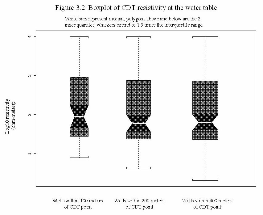
We also created boxplots of the data to look at the distribution of CDT based resistivities at the water table. The boxplots display the shape of the distribution of resistivities at the water table (figure 3.2). It can be see that the median is approximately 1.7 (log base 10 ohm-meters) in both the 200 and 400 meter cases. The mean is drawn to higher values due the positive skew in the data, with data to higher resistivities. This may in part be due to the problems with the digital CDT data that tends to overestimate resistivities. The means are statistically equivalent at the 95% confidence limit, as can be seen by the overlapping notches (or indentations) in the boxplots.
The large variance and skewness of data seen in figure 3.2 indicate that the resistivity at the water table is not well constrained and can not be used as a measure of the location of the water table. This is to be expected. Since the sediment composition varies within the basin, the resistivity of the sediments, whether saturated or not, is based to a high degree on the mineralogical composition of the sediments. Facies changes tend to be more important in controlling resistivity than whether or not the sediment is saturated. Spatial variations in water quality (like salt content) and sediment porosity also can affect the resistivity.
The upper resistivity minimum
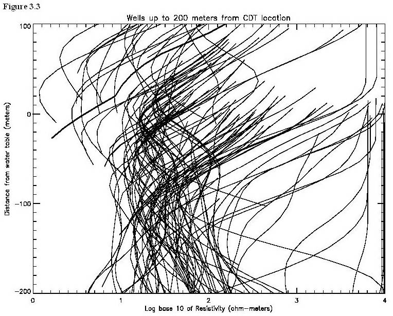
To further test whether the CDT data is useful in locating the water table, we looked at vertical profiles of the digital CDT data at data points closest to, but not farther than 200 meters from, the water wells within the survey area (Tatlow, 1998). These profiles approximate a vertical electric sounding (VES) at each water well. Each of these profiles was positioned vertically by subtracting the elevation of the known water table associated with that CDT vertical profile. The resulting plot, figure 3.3, displays the vertical distance of each profile from the water table on the ordinate and the log base 10 resistivity on the abscissa. In summary, in figure 3.3 each line represents the vertical resistivity profile of a well from the digital CDT data. Zero on the ordinate of the plot represents the water table, positive numbers on the ordinate are above the water table and negative numbers below it. The top of the line represents the elevation of the ground surface.
It can be seen that the first minimum for many lines, the upper minimum in resistivity (as you go down from the top), lies near the water table. We will refer to this feature in the CDT data as the upper resistivity minimum. One might expect to see this relationship in an ideal situation. The sedimentary column is made up of many interfingering facies of sediments that vary from in composition and size. As you move downward towards a point where the pore space is saturated with a conductive fluid, the resistivity may tend to move to a local minimum. It is also possible that the effect is caused by a change in the sedimentary column to a facies that is predominantly clays and silts (which are more conductive than more coarse grain sediments). While many wells display a minimum at approximately 100 meters below the water table, in general it is a second minimum. This represent a lower conductor, probably a zone of clays and silts.
Figure 3.3 indicates that we may be seeing the water table in some of the digital CDT vertical resistivity profile. It is impossible to tell if the minimum resistivity at the water table is due to water table or to the presence of more conductive sediments (or both). In many cases, silts and clays may be supporting the water table. Also, there are many wells which do not display a minimum resistivity at the water table. Based on figure 3.3, it is possible that the minimum resistivity does represent the water table in some of the digital CDT vertical resistivity profiles, but in mant cases the relationship works.
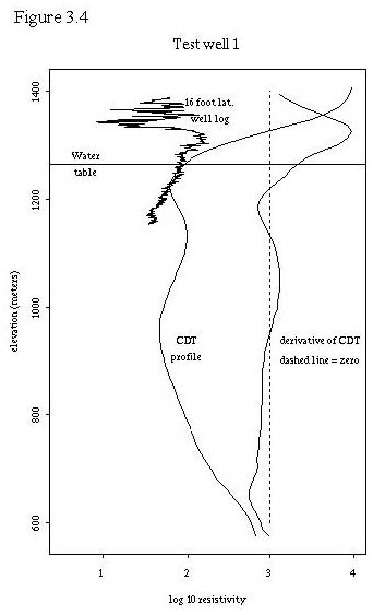
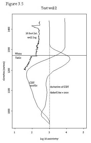
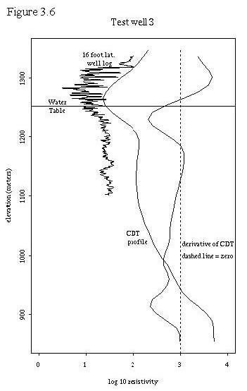
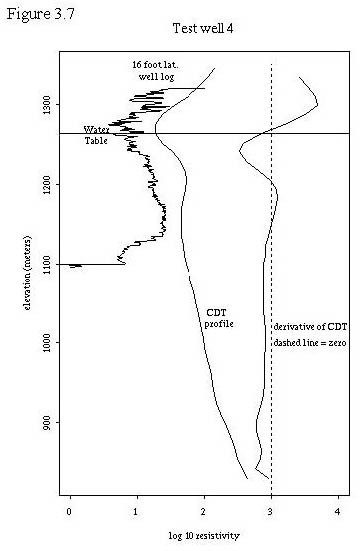
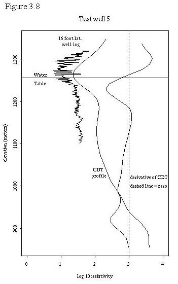
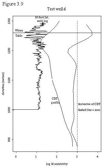
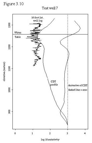
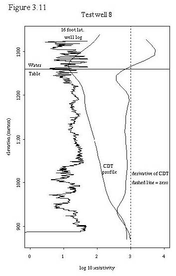
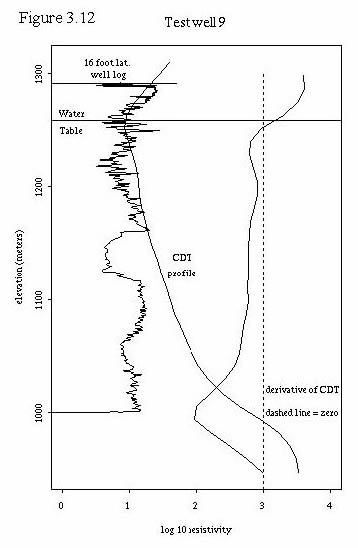
To further test the hypothesis that the upper resistivity minimum may be related to the water table, we utilized 9 test wells where we had resistivity logs (16 foot lateral logs) and water table information. This allowed us to plot the water table, the CDT vertical profiles, and the well resistivity log together for comparison. These 9 plots are shown in figures 3.3 through 3.11. Also, table 3.2 shows the labeling of the test wells in Plate 1 so that their locations can be determined. A general discussion about the plots follows the plots.
Table 3.2
Test well number Well number on plate 1
1 109
2 112
3 96
4 98
5 200 m south of 96
6 82
7 94
8 100
9 97
In addition, a plot of the test wells was created in a fashion identical to figure 3.3, where each digital CDT profile was positioned vertically by subtracting the elevation of the known water table associated with that profile. The resulting plot, figure 3.13, displays the vertical distance of each profile from the water table on the ordinate and the log base 10 resistivity on the abscissa. All test wells wells were within a distance of 200 meters from the nearest CDT point.
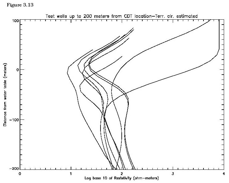
Figures 3.4 through 3.13 demonstrate some interesting relationships between the digital CDTs, the well resistivity logs, and the water tables. First, the digital CDTs consistently demonstrate a higher resistivity at a given elevation than the well log. Part of this difference may be due to the elevation problem that we discovered in the the digital CDTs.
Second, the shape of the CDTs matches the general shape of the well logs in many cases for the first 150 meters depth. That is, if the well logs were to be smoothed with a moving kernel smoother, their shapes would be similar to the CDTs in many cases.
Third, for many of the test wells, the water table lies within a small distance of the upper resistivity minimum. This is not true in test wells 1 and 2 which are drilled in Pantano formation (the other test wells are all drilled in unconsolidated sediments). The digital CDTs at test wells 1 and 2 display extremely high resistivities at the ground level and display an upper resistivity minimum slightly below the water table in test well 1 and about 80 meters below the water table in test well 2. In areas of highly resistive rock at the surface, the upper resistivity minimum does not seem to be correlated to the water table. Test well 6 also displays the upper resistivity minimum below the water table, about 40 meters in this case. All of the other test wells have a digital CDT upper resistivity minimum within one vertical data increment (11.72 meters) of the water table. In general, within the geographic region of the test wells, the digital CDT upper resistivity minimum seems to be fairly well correlated with the water table except when the well is located over the Pantano formation. It is possible that the upper resistivity minimum is due to more conductive, less permeable sediments that control the location of the water table.
Fourth, several observations can be made about the deeper portions of the digital CDT resistivity profiles. The profiles seem to display apparent resistivity; that is, resistivity that is integrated with depth. Thus sections in the digital CDT profiles that are vertical or have a positive slope less than other portions of the curve probably represent more conductive rocks. For this reason, the derivative of the digital CDT profiles are plotted to indicate changes in slope of the profiles. Where these derivatives are zero, or even when they display slight negative slopes, it is still possible to have increasing conductivity in the deeper portions of the profile. In general, the digital CDT resistivity profiles seem well correlated with actual resistivity to depths of 150 meters. At depths greater than this, conductivities seem to be conservatively estimated or underestimated.
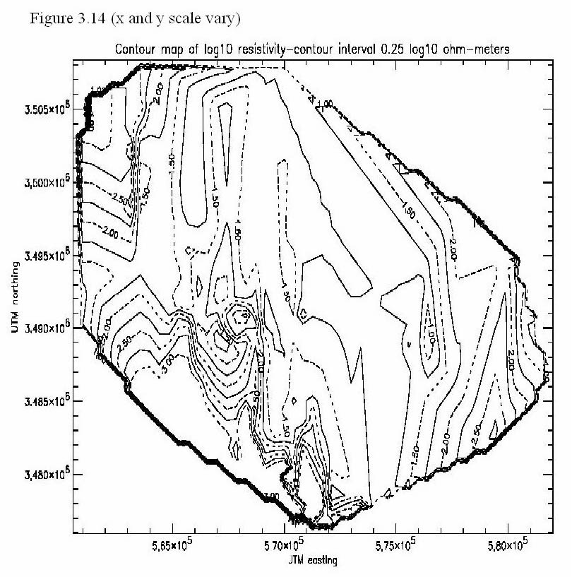
Figure 3.14 displays a contour map of the digital CDT resistivity at the water table of wells that lie within 200 meters of a CDT data point. This map shows that the resistivity, as measured by the digital CDT at the water table, is spatially dependant and is highly correlated to the geology of the upper San Pedro basin. There is a broad area of near constant resistivity in the north central portion of the of the map. This area is underlain by conductive silts and clays that thicken to the east (this is discussed later in this report) and that may control the elevation of the water table. It is in this general region where test wells 3 through 9 are found and the resistivity minimum tends to correlate with the water table. The resistivity increases in the far eastern portion of the map as the bedrock from the Tombstone Hills (see Index Map) is closer to the surface. The western portion of the map has the highest resistivites which are controlled by bedrock from the Huachuca Mountains and by the highly resistive Pantano Formation (where test wells 1 and 2 are located). The low resistivites and tight contours found in the center of the map are due to cultural noise from the city of Sierra Vista as well as a bedrock high in this region that may perch the water table and is described in chapter one of this report.
The upper resistivity minimum map
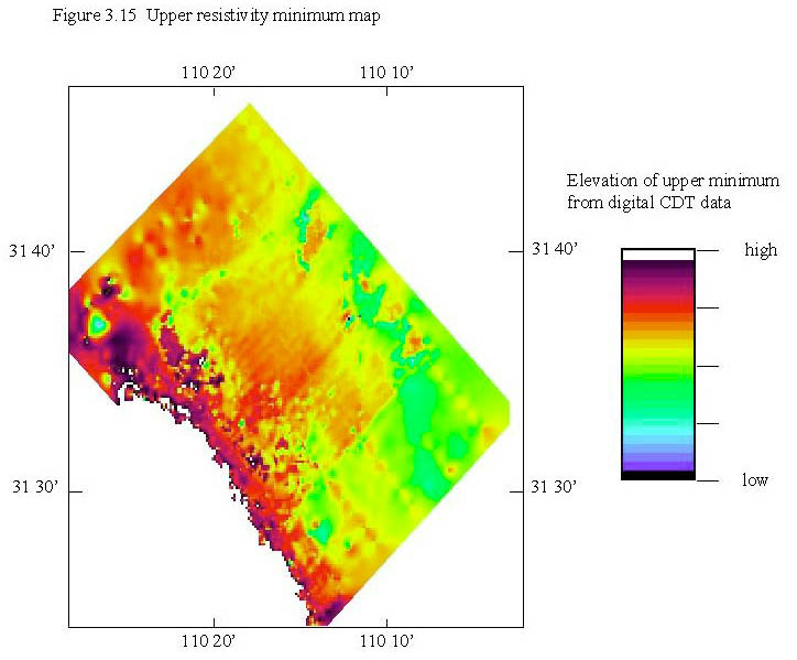
The upper resistivity minimum can be found for all digital CDT data points in the survey, gridded and mapped. The resulting map can contoured or made into an image. If the upper resistivity minimum did represent the water table, such a map would be a good approximation of the water table elevation even in areas where no wells are present. We have seen that in the upper San Pedro basin, the water table seems to be well correlated to the upper resistivity minimum when compared to some wells, but not to all wells. Also, even where the upper resistivity minimum and water table are well correlated, it is impossible to determine if it is the water table or the presence of silts and clays that are causing the minimum. One way to further test the feasibility of using the upper resistivity minimum to locate the water table is to create an upper resistivity minimum map and compare it to the known water table. The upper resistivity minimum map for the 1997 San Pedro AEM survey is shown in figure 3.15.
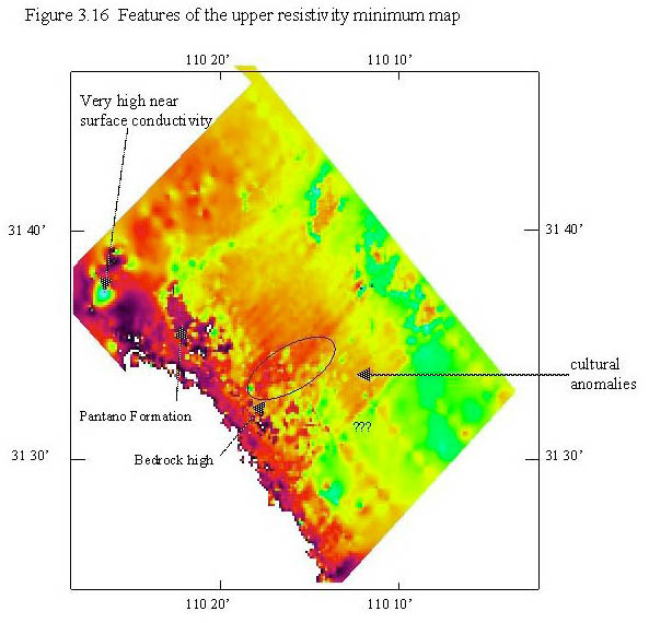
There are some interesting features in the upper resistivity minimum map that bear pointing out. These are summarized in figure 3.16. First, a combination of high and low values in and around the Sierra Vista area is noticeable. These are due to cultural noise in the area to the west of the arrow leading from the "cultural anomalies" label on figure 3.16. In the Sierra Vista area, magnetic and gravity survey data (from Chapter 1) indicates that there is a bedrock high, located by the ellipse. If the AEM data is seeing through the cultural noise at all, it indicates that this bedrock high may perch the water table. Many of the other speckles leading from western Sierra Vista through Fort Huachuca to Huachuca City are also probably due to cultural interference in the AEM data.
The very resistive Pantano Formation is clearly visible as very high elevations in the image (figure 3.16) and is indicated by an arrow. North and east of the Sierra Vista bedrock high is a region of clay and silt sediments that keep the upper resistivity minimum (and possibly the water table) high. It is in this region that the upper resistivity minimum was highly correlated with the water table in the test wells. To the west of this region, and to the east of the indicated Pantano Formation, is an area of lower elevation for the upper resistivity minimum. This region may be related to the thinning and disappearance of clays and silts and/or to a lowering water table.
The area labeled "Very high near surface conductivity" can be seen in cross section in CDT number 102 in Plate 3.1. In this region there is very conductive layer near or at the surface that confuses the algorithm that locates the upper resistivity minimum. In this area, ground water may be confined by structural features and lies very near the surface (B.B. Houser, oral communication, 1998). The area labeled with the three question marks ("???") represents a region where there is likely a structural feature but it can not be precisely resolved because the 400 meter spaced data ends just to the northwest.
Due to the number of cultural anomalies, the minimum resistivity map was smoothed using an algorithm that looks at all points within a circle of radius 500 meters, averages them, and generates a new data point. The smoothed upper resistivity minimum map is shown in figure 3.17. It does help remove a number of the anomalies present in figure 3.15, yet the values of smoothed regions are still affected by the anomalies.
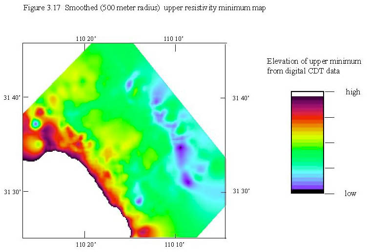
In order to compare the upper resistivity minimum map with the water table, we decided to use the smoothed map which minimized cultural anomalies. The 1998 well water level data (Tatlow, 1998) was gridded with a minimum curvature routine to produce a water table grid. The smoothed upper resistivity minimum map was then subtracted from the water table grid resulting in figure 3.18, shown below.
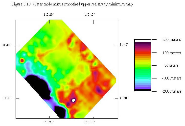
Figure 3.18 shows that the upper resistivity minimum map does a good job of approximating the water table in the central portion of the basin. In the west, where resistive high energy facies rocks are present, it tends to overestimate the elevation of the water table. In the east, it tends to underestimate it. The water table is drastically underestimated in the south central portion of the map (where the water table minus the upper minimum resistivity map approaches 200 meters) for unknown reasons.
Conclusions on the relationship between the digital CDT data and the water table
While the upper resistivity minimum of the digital CDT resistivity profiles serves as a good approximation of water table elevation in some regions of this study, it does not work well in all regions. Also, it is unknown if the upper resistivity minimum is due to the water table or to clay and silt facies in the sediments in the places where it does work. While this methodology can be used to approximate the elevation of the water table in regions with no water wells, the actual water table as measured from well water levels should be used in the upper San Pedro basin. Further study on methods of transformation or inversion and methods to remove cultural noise may help define what the AEM data is actually seeing.
The structure and sediment fill of the Upper San Pedro basin based on digital CDT data
The data cube consists of two blocks of data due to the two different directions of flight lines. The data from flight lines 101 through 159 was put together into one data cube block, referred to as block 1. Between the 1600 meter spaced data, CDTs were built at a 400 meter spacing by a distance weighted average of the CDTs on either side. A line perpendicular to the average CDT line direction was draw through the origin of CDT 110 and this line serves as the southwest margin of block 1. The CDTs were then assumed to be parallel and exactly 400 meters apart (which introduce only some small x-y small errors, infrequently more than about 50 meters) and interpolated for differences in the down flight-line distances between sample points. The result is a data cube with data of known spacing in the x, y, and z direction. For block 1, the x spacing (along flight lines) is 46.13 meters, the y spacing is 400 meters and the z spacing is 11.72 meters.
The data from flight lines 5001, 6001 through 6010, 5002 was put together in a second data cube block referred to as block 2. This data cube has an x spacing (along flight lines) of 46.38 meters, a y spacing of 400 meters, and a z spacing of 11.72 meters. It should be noted that the x and y coordinate system is set in each block so that the x direction moves along flight lines and y is perpendicular to this. So, the x and y coordinate system of blocks 2 is rotated approximately 90 degrees with respect to block 1.
It should be recalled that the original digital CDT data has elevations errors. Due to time constraints, only the average radar altimeter value was used to correct this in the volumetric data. This means that in the area of the survey with high relief, the elevation of the data values may not be accurate. These errors should have little effect on making conclusions about the structure and sedimentology of the upper San Pedro basin.
The volumetric data is extremely useful for looking at the digital CDT data in ways or orientations that are different from the resistivity cross sections that can be built along each flight line. So, the figures which follow will look at horizontal or oblique slices through the data cube and at vertical slices that are perpendicular to the flight line direction in a block. The data along flight lines can be seen by simply looking at the CDTs for each flight line (plate 3.1, plate 3.2, plate 3.3, plate 3.4) and when necessary, these CDTs will be referred to by number.
Figure 3.19 is a horizontal slice at an elevation of approximately 980 meters through block 1 that is viewed from above looking in an approximately northerly direction. North is up. The point labeled "(0,0,0)" is the origin for block 1, the northwestern corner of the data cube. The x axis, which is along the flight line (spacing = 46.13 meters), goes from the origin to the northeast. The y axis (spacing = 400 meters) goes from the origin to the southeast. The z axis (spacing = 11.72 meters) goes up (vertically). Areas that appear black in the interior of the slice are places where the CDT data set contains no information.
The highly resistive bedrock of the Tombstone Hills (see Index Map)can be seen to the northeast. In the southwest, the distance from ground surface to the elevation of this slice is large and the CDT data cube here contains no information. A northeast trending linear feature can be seen in the eastern portion of the data slice. It is a very conductive surface feature (an aqueduct) that prevents the AEM system from making observations at depth. Also, at this elevation it can be seen that the sediments on the west side of block 1 are more resistive than those on the south side of the block.
Resistivity is in log base 10 ohm-meters.
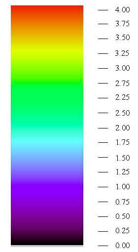
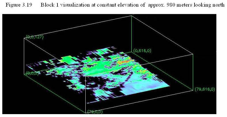
Figure 3.20 is a visualization from the same observation point, but looking at a slice taken at an elevation of 1223 meters. The bedrock associated with the Tombstone Hills is now more apparent on the northeast side of the block. Also, the nature of the resistivity of the sediments in the basin has changed. The sediments that are close to, but not abutting, the Tombstone Hill bedrock are very conductive, probably silts and clays deposited from the Tombstone caldera (Moore, 1993) in a low energy environment. These grade to the west to more high energy, more resistive, sedimentary facies. There is still no CDT information under the Huachuca foothills, the city of Sierra Vista, and the aqueduct (see Index Map).
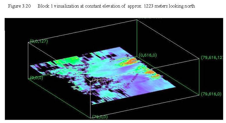
Figure 3.21 is a visualization again seen from the same perspective as the previous two figures but it displays a horizontal slice at an elevation of approximately 1320 meters. The elevation of this slice is above ground level for the east side of the basin. As in the previous figure, the resistivity of the sediments at this elevation decreases to the east and at the eastern margin of the data is very low. At the eastern margin, the resistivities are lower than in figure 3.20 (which is deeper) indicating that resistivity appears to be decreasing with shallowing depth, This may be an artifact due to the CDT's tendency to integrate resistivity with depth. Another region of low resistivity can be seen in the central portion of the data that is displayed, approximately under the city of Sierra Vista (see Index Map). This may be due to cultural noise or to the bedrock high, discussed previously, that lies in this region. The high resistivity regions are the lower portions of the Pantano Formation. This elevation slice intersects some of the high resistivity rocks of the Tombstone Hills at the northeast margin of the block.
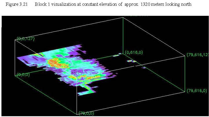
Figure 3.22 is from the same observation point as the previous three figures, but now uses an oblique slice whose dip to the east approximates the dip of the topography. This slice summarizes most of the information in the first three visualizations except that Pantano formation rocks can not be seen. The eastward decrease in resistivity of sediments can be clearly seen in figure 3.22. CDTs 101 through 159 (plates 3.1, 3.2, and 3.3) clearly show the increasing thickness of these less resistive units to the east.
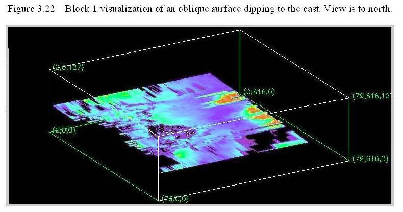
Figure 3.23 is a visualization of block 1 looking to the north-northeast. The block has been rotated slightly counter-clockwise from the previous four visualizations. In this visualization, vertical slices are drawn perpendicular to the direction of the flight lines. Starting at the southwest most line, the resistive rocks of the Pantano formation are clearly visible. As you move to the northeast, a thin layer of conductive rocks becomes visible in the second slice. This layer is the upper resistivity minimum and may be related to the water table in some locations. Variations in the level of this conductive layer near the northwest end of the line may be associated with water table depression. The conductive layer becomes thicker to the east up to the bedrock associated with the Tombstone Hills (see Index Map). The Sierra Vista bedrock high (unless this feature is due to cultural noise) can be seen in the second slice from the southwest side of the block. The northeast-most slice in figure 3.23 display high angles relationships between sediments and the bedrock of the Tombstone Hills. This is due to the complex structure and stratigraphy of the Tombstone caldera mapped in this region (Moore, 1993).
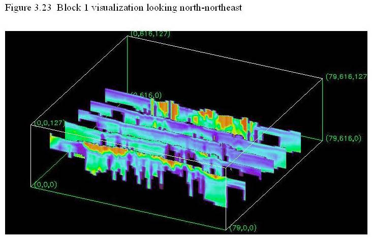
Figure 3.24 is a visualization from a position identical to 3.23 but includes more slices that are in slightly different locations. It displays many of the features seen in figure 3.23. In addition, it shows what may be complex patterns of faulting in the Huachuca Mountains foothills, on the southwest side of the data cube.
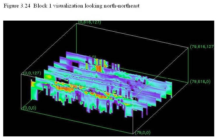
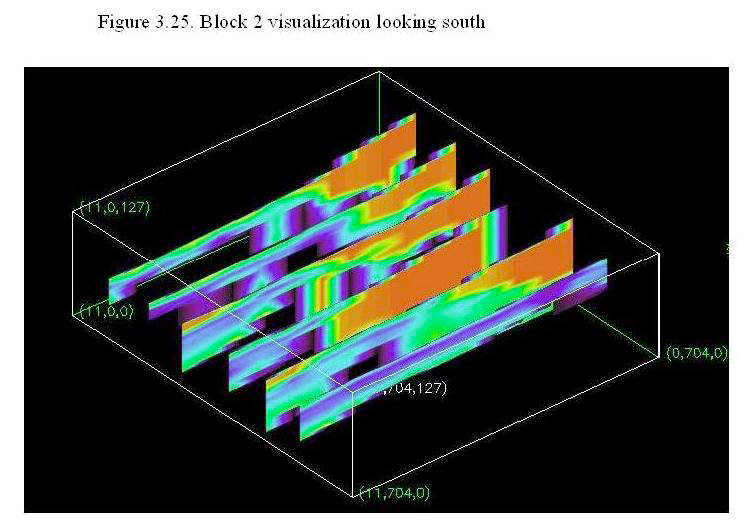
Figure 3.25 is a visualization of block 2 looking to the south from the over the northern corner of the block. The x axis (data spacing 46.38 meters along flight lines) extends to the left of the point labeled "(11,704,0)". The y axis (data spacing 400 meters) extends to the left of this point and the z axis (data spacing 11.72 meters) extends up from this point. While there are only 12 flight lines in this data cube, some important features can still be seen. The area of high resistivity on the top of the left side of of the slices is Pantano formation. The large high resistivity area in the center and right portion of the slices is Pre-Cambrian granite in the Huachuca Mountains foothills. The basin bounding fault to the left (northeast) of the granite can be clearly seen. A low resistivity region under the Pre-Cambrian granite may be evidence for a fault under or within the granite body that coincides with a mapped thrust fault (see Plate 1).
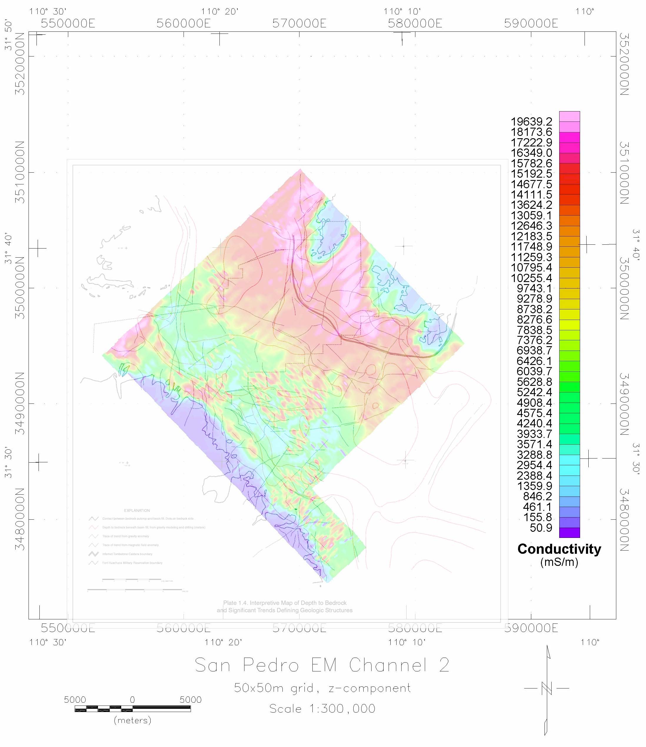
Comparison of potential field and AEM analyses
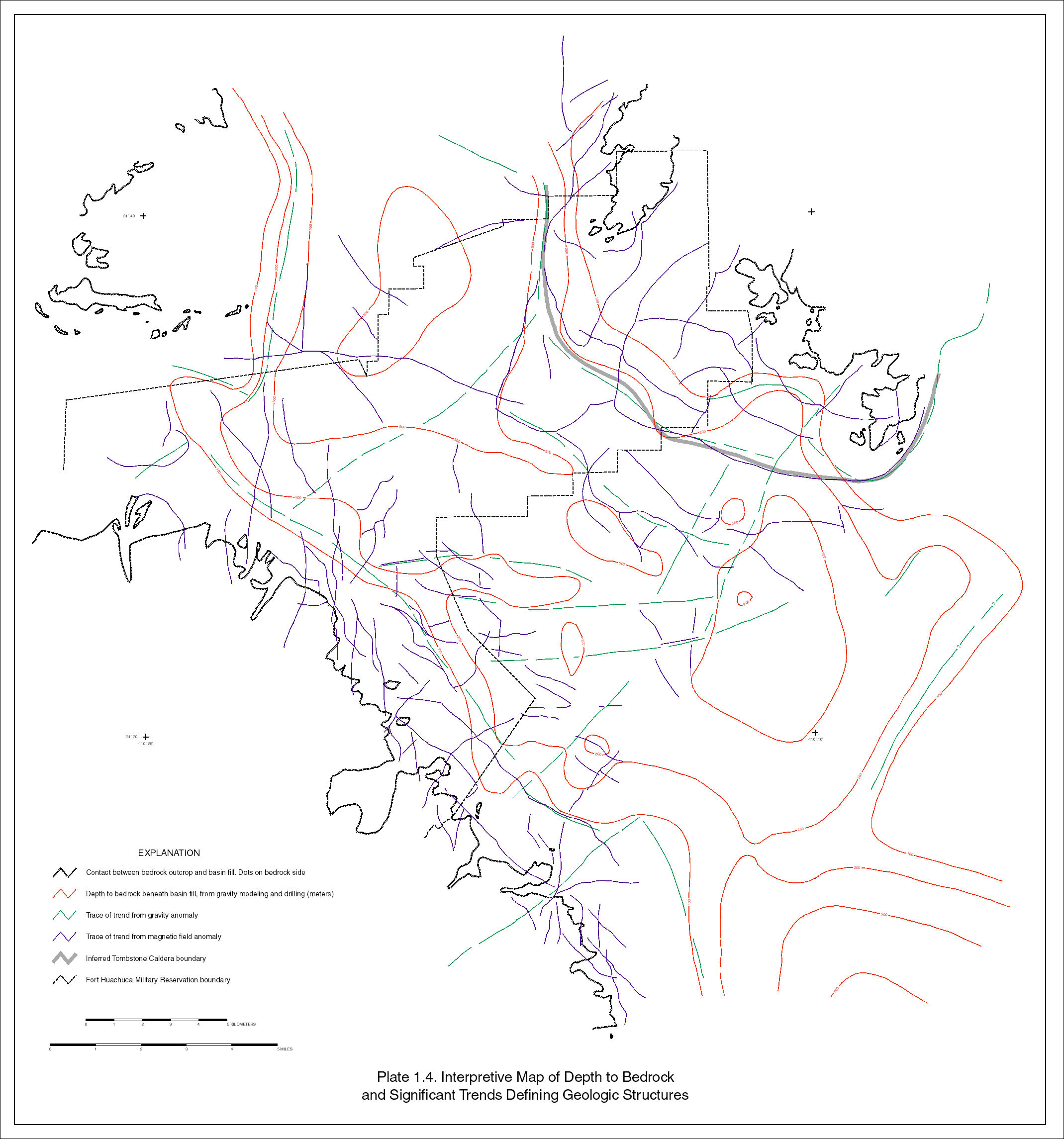
Figure 3.26 shows an overlay of Plate 1.4 (Chapter 1) summarizing the potential field data interpretation on Figure 3 from Chapter 2 (gridded Z component of AEM channel 2). Study of figure 26 shows many correlations between the deep electrical conductors and inferred structure from the potential field data. The Tombstone caldera margin inferred from the gravity and magnetic data divides a deep region of high conductivity within the caldera from lower conductivites outside the margin. Many of the magnetic and gravity anomaly trends correspond to nearby breaks or offsets in the conductivity map. Further study of these relationships is warranted.
Conclusion about the structure and sediment fill of the upper San Pedro basin based on digital CDT data
The digital CDT data is reliable only to a depth of about 150 meters, less in areas of low resistivity material at the surface. There is some information below this depth in areas with highly resistive surface rock, but the CDT algorithm tends to integrate resistivity at depths below 150 meters. In general, information on the bedrock under the basin sediments is not visible in the CDT data except near where the bedrock outcrops.
Given the assumption that clays and silts occur together and that they are more conductive than sands and gravels, a few conclusions can be made about the basin structure and geometry based on the digital CDT data. The upper San Pedro basin is bounded on the southwest by a high angle fault near the edge of the basin. Magnetic and gravity data (Chapter 1) point out a bedrock high in the Sierra Vista area that extends to the east about 10 kilometers into the basin. This feature can also be seen in the CDT data as a near surface conductor. South of the bedrock high the basin is complex, but seems to be shallower than north of the bedrock high. To the east of the basin bounding fault near the Huachuca Mountains and east of the Sierra Vista bedrock high, the basin remains deep until it approaches the Tombstone Hills. The relationship between the basin sediments and the bedrock in the Tombstone Hills area is complex and may be both stratigraphic and fault bounded. This region correlates to the mapped Tombstone caldera (Moore, 1993).
The sediment fill in the basin contains many interfingered layers of clays and silts with coarser grained material. In general though, the thickness and amount of fine grained, low energy environment derived material is higher on the eastern edge of the basin. This zone thins towards the west. On the western edge of the basin, the dominant fill material is likely the gravel, sand, and unconsolidated material that is mapped at the surface.
References

![]() U.S. Department of the Interior |
U.S. Geological Survey
U.S. Department of the Interior |
U.S. Geological Survey
URL: http://pubsdata.usgs.gov/pubs/of/1999/0007-b/bultman/ch3.html
Page Contact Information: GS Pubs Web Contact
Page Last Modified: Wednesday, 07-Dec-2016 17:50:57 EST
