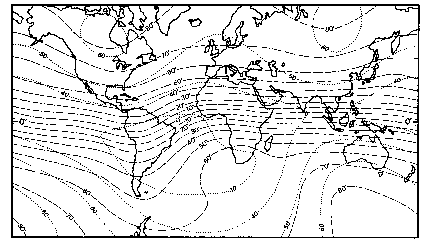
The Earth has a dipolar vector magnetic field that originates in the core. In Alaska the magnetic vector dips steeply (between 70 and 80 degrees) and has a magnitude between 50,000 and 60,000 nanoteslas (figure from Milsom, 1996).

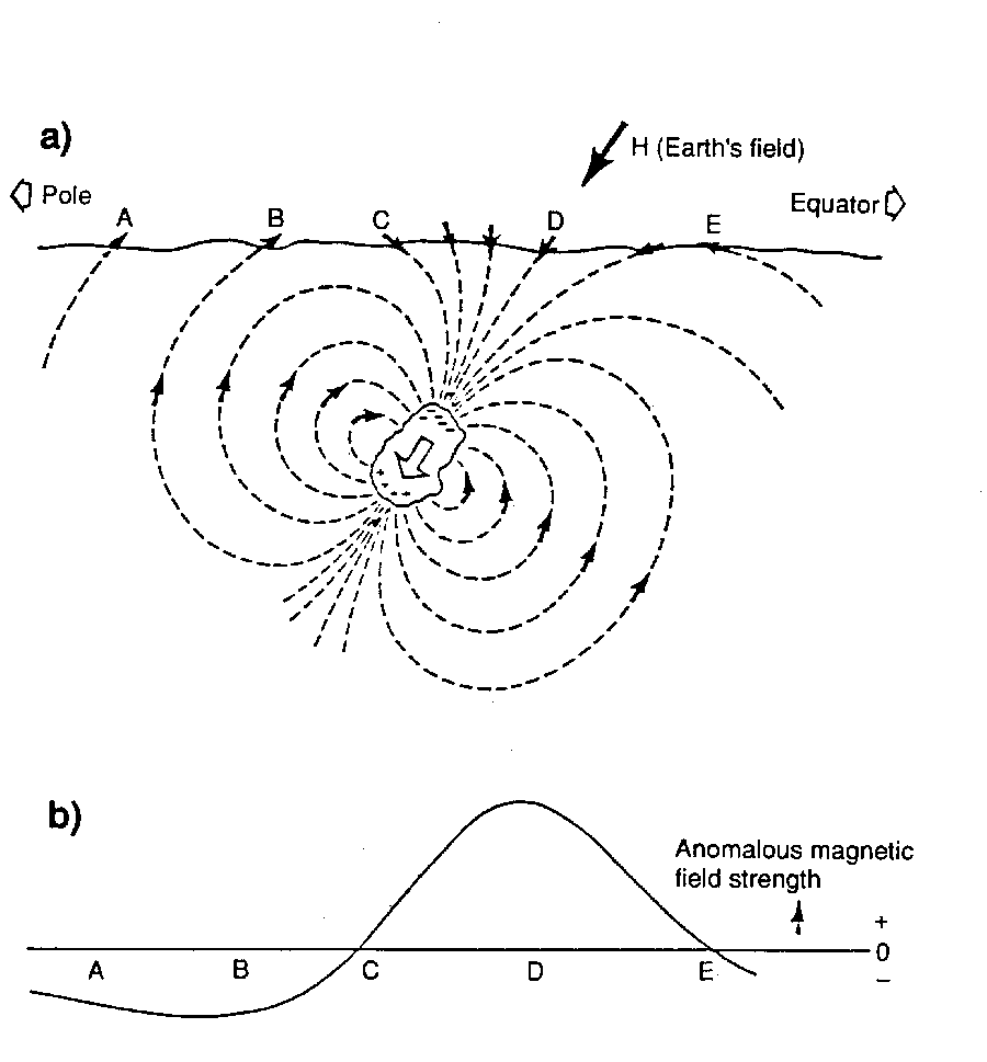
The presence of magnetic minerals in rocks causes distortions in the Earth's magnetic field. This picture shows the induced field created by a magnetic rock. At D the induced field adds to the Earth's field and causes a high anomaly. At B the induced field acts against the Earth's field and causes a low (figure from Milsom, 1996). Note that the inclination of the magnetic field (the angle that the Earth's field strikes the surface) in most of Alaska is steeper than depicted here.

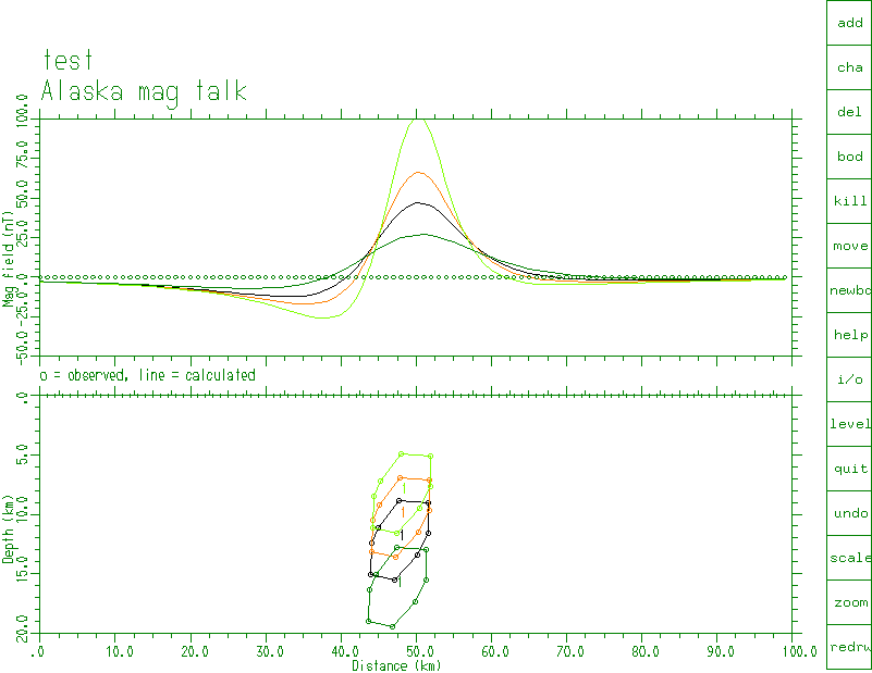
Here is a picture from a program for calculating the magnetic anomaly for simple geometrical bodies. The calculated anomaly curves are color-coded to the bodies that caused them. Deeper bodies cause broader, lower amplitude anomalies. Shallower bodies cause sharper, higher amplitude anomalies. The bodies in this example are two-dimensional: they extend to infinity in and out of the page.

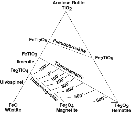
The primary magnetic minerals that cause magnetic anomalies are part of the Ulvospinel-magnetite solid solution series. Other iron-bearing minerals are important in local settings, particularly for high-resolution magnetic studies (Reynolds and others, 1990).

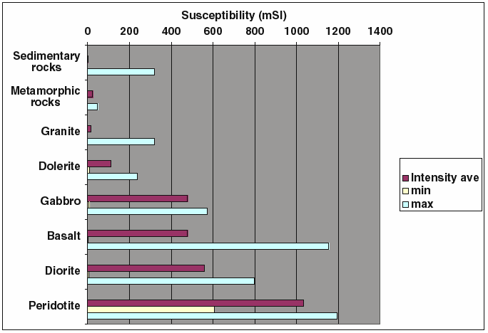
Magnetic susceptibility is the physical property that determines how much induced magnetic anomaly a body of rock will produce. In general, sedimentary rocks have relatively low magnetic susceptibility, as do most metamorphic rocks. Igneous rocks tend to be more magnetic, with more mafic rocks having generally higher susceptibility than more felsic rocks. We expect, on a regional scale, that oceanic crust will be more magnetic than continental crust. Susceptibility values are from Telford and others (1976) and Carmichael (1982).

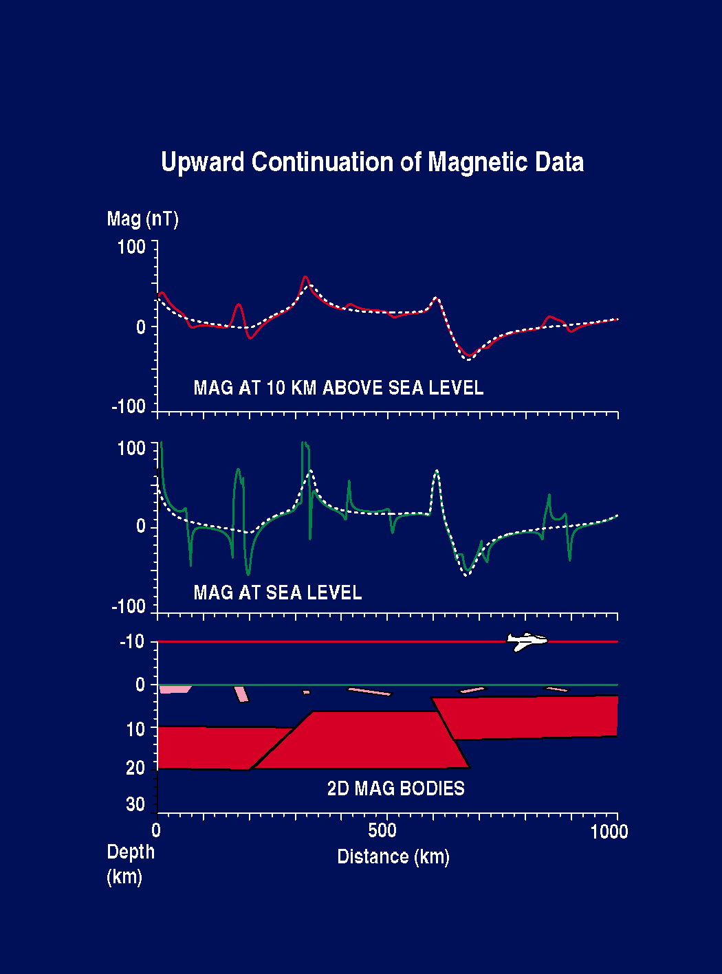
Magnetic anomaly maps, such as the map of Alaska described in this report, contain features that originate from a wide range of depths. One technique to isolate deep versus shallow sources is through the use of upward continuation. This slide shows how a survey measured at sea-level differs from a survey measured at an elevation of 10 km. In each panel, the white dashed line indicates the anomaly caused by the deep sources; the colored curve is the complete anomaly (shallow plus deep sources). At sea-level the shallow sources dominate. At 10 km, the crustal-scale sources dominate. We do not have to collect data at two elevations - we can use the mathematics of potential-field theory to convert surveys from one level to another. Downward continuation enhances noise and is complex - upward continuation is a smoothing operation and is easier.