Two areas were modelled in this way. The Surprise Spring Basin and Deadman Lake Basin were included in one model and the Yucca Valley - Joshua Tree - Copper Mountain College area in another (referred to here as the Joshua Tree Basin).

Bedrock grid from generalized geology map. Red indicates pre-Cenozoic basement rocks where computed basin depth must be zero. Yellow indicates areas of lower density sediments where the program computes depths.

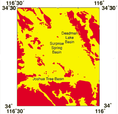
This first illustration shows the generalized geology grid of the area of the gravity map. Portions of this were used for the two depth to bedrock computations.

Results of depth to basement computation for the Surprise Spring and Deadman Lake basins.

A new estimation of the thickness of Cenozoic deposits (depth to granitic basement) in the southern part of the Twentynine Palms MCAGCC was made based on a new compilation of gravity data, drill hole information, and outcrop geology. The area of interest is centered over the Surprise Spring basin and the basin adjacent to it on the east (Deadman Lake basin), between the Surprise Spring (Hidalgo) fault and the Bullion Mountains.

The study area coincides with that studied by Moyle (1984) but the number of gravity stations in the present study is more than twice that used in the earlier study, more gravity stations are used to define the gravity field of the granitic basement, a number of detailed gravity profiles cross the Surprise Spring fault. This provides a detailed image of the geometry of the basement surface where cut by the fault, and thus an estimate of the vertical offset across the fault, at least since the Cenozoic sediments were deposited. Wells that penetrated granitic basement are used explicitly in the inversion to constrain the solution, and the inversion is fully 3-dimensional, thus providing much more detail in the map of sediment thickness and the geometry of the basement surface.

We used 5 density contrasts of -0.40, -0.35, -0.30, -0.25, and -0.20 g/cm³ relative to the 2.67 g/cm³ used for the gravity data reduction with bottom depths of 50m, 100m, 150m, and 300m. Eight wells (one just to the west of Fig. 1) that penetrated the basement were used to constrain the model. This density depth structure was adopted by starting with density/lithology information from wells and adjusting the structure with each run so the basin thickness computed without well constraint more closely matched that with well constraint.

Note that there is poor well constraint on the Deadman Lake area and it is highly likely that the basin is shallower than indicated with thicker layers of the lower density fill. To see map (Fig. 1) click here. (148 K).

Many of the features seen on the new sedimentary thickness/basin depth map reflect features on the surface of the granitic basement. A number of these features also are seen crudely on the coarse aeromagnetic data over the area. A high resolution aeromagnetic map could refine the locations and geometries of many of these features, including the Surprise Spring and Emerson faults, and the deep basins throughout the area.

RESULTS

Surprise Spring (Hidalgo) fault

The Cenozoic sediment thickness map provides insights into characteristics of the Surprise Spring fault, the fault that separates the Surprise Spring ground water basin from the basin to the east, here informally called the Deadman Lake basin. The new information relates mainly to the possible offset on the fault, and thus indirectly to the likelihood of the fault moving in the future and the possible effectiveness of it as a ground water barrier.

The sediment thickness map reveals a narrow east-west channel in the top surface of the granitic basement (labeled C) that connects the shallow basin along the Emerson fault about 3 km NNW of Sand Hill (A) with the Deadman Lake basin to the east (B). This channel also is seen in the coarse magnetic data we have over the area. The buried channel is parallel to and about 1.5 km south of the present drainage at Surprise Spring. This channel crosses the Surprise Spring fault about 1 km south of Surprise Spring but is not obviously deflected at the fault, suggesting that any strike-slip offset on the fault has been very small, at least since the beginning of sedimentation onto the granitic basement. No strike-slip offset is required by the present data but, based on the gravity station distribution, perhaps as much as 500 m of right-lateral offset could be present and not violate the data. In any case, very little strike-slip offset has occurred during the past few million years (or however old the oldest sediments are). By comparison, the fault that ruptured during the Hector Mine earthquake (north of this area) shows 3.4 km of total offset, and the faults that ruptured during the Landers earthquake (west of this area) show 3-3.5 km of total offset.

The change in thickness of the sediments from one side of the fault to the other should provide a measure of the amount of dip-slip offset accommodated across the fault since the beginning of sedimentation. As with the strike-slip offset, the inferred dip-slip offset appears to be very small. From Surprise Spring north along the fault, the change in sediment thickness across the fault is small (much less than 150m (500 ft)) and inconsistent in polarity (as shown by the u-d symbols indicating inferred u-upthrown side, d-downthrown side). Interestingly, along this stretch, the prominent abrupt change in sediment thickness that might indicate the location of a basin-bounding fault (D) lies not along the Surprise Spring fault, but about 1-1.5 km to the east. South of Surprise Spring, the change in thickness across the fault suggests dominantly down-to-the-east with an average magnitude of about 150 m (500 ft). This magnitude is slightly less than implied on figure 1, but includes an approximate correction for surface topographic effects.

Thus the inversion presented in the figure implies that the Surprise Spring fault has not experienced much movement, either strike-slip or dip-slip, at least since the last time the basement was exposed. In particular, it seems to have experienced less movement than the surrounding, recently active faults on which the Hector Mine and Landers ruptures occurred. Thus its earthquake potential seems to be substantially smaller than its adjacent neighbors. Despite this, water levels show that the Surprise Spring Fault is a significant ground water barrier.

The basin a few km NNW of Sand Hill (A) is shown in the present results to be bounded by linear, abrupt changes in thickness of the sediments on the NW and NE. These linear features suggest faults, probably associated with the Emerson fault system.

North and east of Surprise Spring, the large basin (B on Figure 1) is seen to be compound, with a shallow basin 1-2 km east of the Surprise Spring fault, and separated from the extremely deep Deadman Lake graben by a weak basement ridge. The Deadman Lake graben is likely a strike-slip extensional basin caused by a right slip across a right step from the Mesquite Lake fault to the Bullion Mountains fault.

Results for the depth to basement computation for the Joshua Tree basin.

A series of basin thickness models was generated based on different sets of assumptions. Only a few wells were known to penetrate the basement rocks and information from some of the older wells is suspect. Well logs of other wells show they did not reach basement rocks and there are many other wells where such information is not available and some of them go deeper than the computed basin depths of the shallower models in some areas. Northwest of Yucca Valley the gravity low (without constraint by basement gravity stations) extends into the basement rocks. No attempt was made to account for this in the models thus the plots show significant basin depths directly adjacent to the edge of the basin.

While the models differ in the computed depths, they are very similar in shape and conclusions drawn from one may be applied to the others. All models show an east-west linear basin parallel to and including the Pinto Mountain Fault and a second basin north of that in the Coyote Lake area with a slight buried ridge between them.

The first model was run with a single density contract of -0.55 g/cm³. This may be considered the most extreme case and yields the shallowest depths. In addition to the shallowest maximum depths (~4200 ft or ~1280m), this model has the most unknown wells penetrating the computed basement surface, and is probably unrealistic. Click here to see the results of model 1 (Figure 2, 68 K).

A second possiblilty is a density profile similar to that in the Surprise Spring area with density contrasts of -0.40, -0.35, -0.30, -0.25, and -0.20 g/cm³. We used depths of 100m, 200m, 300m, and 500m for the upper layers. This model is the best in some of the shallower areas such as north of Joshua Tree suggesting that in those areas there is less of a density contrast with the adjacent rocks. Even with this model there are several wells that penetrate the computed basement surface yet claim to bottom in fill.The drawback to this model is the extreme depths (a maximum of about 12000 ft or 3700 m) generated in the deeper portions of the basin. Click here to see the results of model 2 (Figure 3, 72 K).

A third model assumed a density depth profile similar to that used by Biehler (1988) with contrasts of -0.70, -0.40, -0.35, -0.30 g/cm³ with depths of 70 m, 300 m, and 400 m. Click here to see the results of model 3 (Figure 4, 88 K).

A fourth model was that used for Nevada (Jachens and Moring 1990) with density contrasts of -0.65, -0.50, -0.35, -0.25 g/cm³ and depths of 200 m 600 m, and 1200 m. Click here to see the results of model 4 (Figure 5, 84 K).

These models differ in computed depths but are very similar in the configuration of the basins and the relative depths of various portions of the basins. Maximum depths in feet given by the 4 models are as follows:

Based on the available information, some combination of model 2 (shallower areas) and either 3 or 4 (deeper areas) is probably the most realistic.