Illinois State Geological Survey
615 East Peabody
Champaign, IL 61820
Telephone: (217) 244-0365
Fax: (217)333-2830
e-mail: johnston@isgs.uiuc.edu
Tazewell County covers an area of approximately 600 square miles in central Illinois. The county is bordered on the west by the Illinois River, and is bisected by the east-west-trending Mackinaw River. The surficial geology of the county is varied; the eastern half is covered by thick Wisconsin-age glacial tills, and the western half is covered by Wisconsin-age and younger outwash and fluvial deposits. Tazewell County is a predominantly rural county, but its western areas are experiencing urban encroachment from the city of Peoria.
The arc and point coverages from the 20 quadrangles were reprojected to a common projection and datum and merged. TopoGrid was used to create a 30-foot grid, with stream and lake coverages (collected from the same sources as the hypsography) used to control valley shapes. ArcMap was used for inspection of the grid, and editing of the original coverages was performed several times to correct misplaced or mislabeled features. Contours were created digitally using the CONTOUR command in ArcGrid. To reduce pixelizing, or "grid-tracing," of contours, the contour interval was set to 10.001 feet. The resultant line coverage was corrected for topology using ArcEdit, and some manual and digital generalization was performed to make contours appropriate for display at a scale of 1:62,500. The HILLSHADE and SLOPE functions in ArcGrid were used to create shaded-relief and surface-slope grids.
Three maps were created directly from these data (Surface Topography, Shaded Relief, and Surface Slopes), and all layout and presentation were performed using ArcMap. An interesting problem that emerged during layout was the inability of ArcMap 8.1 to properly label contours. The traditional technique of blanking out a section of contour line under the label can only be performed in ArcMap by using a "halo" around the label. However, this "halo" effectively blanks out any underlying themes (e.g., elevation color bands, thematic polygons). The only practical solution found for this problem was to export the contour layer into Adobe Illustrator, insert labels, then return the layer to ArcMap -- a cumbersome procedure for what should be a simple step in the map-making process.
The data source for 3-D modeling was the ISGS Well Log Database. This database stores location information and well-drillers' lithologic descriptions for most water wells, engineering borings, oil and gas exploration wells, and research borings drilled in the state. For Tazewell County, more than 5,000 well records exist.
The well records for Tazewell County were first checked for locational accuracy. For those not located within a quarter-quarter-section (approx. 330 feet), the driller's location description was compared to topographic maps, aerial photography, and plat maps to refine the location. If the location information was inconclusive, the data from that well were discarded. As a second location-accuracy test, reported elevations of all remaining wells were compared to spot elevations from the 30-foot DEM produced for the project. If the reported and spot elevations differed by more than 10 feet, the location and elevation data were scrutinized, and the well location was moved or the elevation was adjusted. If there was no satisfactory remedy, the well data were discarded.
For the accurately located wells, the lithologic descriptions were classified into five grain-size categories (fine, mixed-fine, mixed, mixed-coarse, coarse) or as bedrock. The reclassified lithologic records were then viewed in ArcView using the 3D-Analyst extension. The top of each unit in the well was assigned an elevation and the thickness data were used to compute the unit's 3-D geometry (to be shown with 30X vertical exaggeration). One-mile-wide "strips" of the wells were viewed in 3-D, first east-to-west, then north-to-south. These "virtual cross sections" were useful in helping to locate spurious data, and in reconciling records that were inconsistent with nearby data.
The result of these editing/quality control steps was a reliable data set that provided accurate data input for the modeling and made post-model editing of the data set less necessary. Although more than 20% of the available data was discarded, approximately 23,000 data points from over 4,000 wells were used in the final modeling process.
Data on depth-to-bedrock was collected from the well records used for the 3-D modeling. Just over 400 wells reported reaching bedrock, and these were used to create an elevation grid. The grid was further enhanced by comparison in 3D-Analyst to 400 wells that did not report bedrock but pierced the surface of the preliminary bedrock-surface grid. These wells were used to "push" the surface downward where appropriate to a depth equal to the well depth plus 5 feet. Additional depth-to-bedrock data came form an earlier study covering the southeastern corner of the county (Herzog and others, 1995).
Once the final bedrock-surface grid was created using TopoGrid in ArcInfo, ArcGrid was used to subtract this grid from the land-surface grid previously produced, creating a drift-thickness grid. These grids were contoured using the CONTOUR command in ArcGrid, and the line work was manually generalized to make contours that were appropriate for display at the 1:62,500 scale.
Several factors were considered when sensitivity classes were assigned to certain depth/thickness categories. The classes represent sensitivity of the aquifer to application of contaminants (1) at the surface (such as agricultural chemicals), (2) in shallow trenches (septic fields, etc.), or (3) in deeper trenches (landfills). The classifications deal with aquifers when the top of the aquifer is within 100 feet of the land surface, representing a maximum depth for infiltration of materials applied at the surface, while also recognizing that modern landfill processes commonly include trenching more than 30 feet into the subsurface.
Although the classification scheme for Tazewell County did not include aquifers with tops below 100 feet, an inset map was included to show where aquifer materials were present below this depth. In the map area, there are two major preglacial valley systems that intersect, and both are partially filled with thick proglacial sand and gravel deposits. These deep aquifers represent an important local and regional ground-water resource.
The Aquifer Sensitivity Map was created from a 3-D solid model that was generated with EarthVision software. The reviewed and edited well-log data were used to generate a 3-D solid model, and regions of coarse (sand and gravel) and fine (loam, silt, and clay) sediments were delineated. The coarse material was designated "Aquifer Material" and the fine and mixed units were designated "Non-Aquifer Material." This model was sliced into layers, each representing depths found in the classification scheme (0-5 ft, 5-20 ft, 20-50 ft, 50-100 ft, 100+ ft below ground surface). For each layer, an isopach map was generated which displayed the thickness of aquifer materials present in that layer. These coverages were displayed over images that showed the materials present at the top of each layer. By analyzing these displays, the top and thickness of each aquifer unit could be determined, regardless of whether the unit was wholly contained within one layer, or extended through several layers.
An ESRI polygon coverage was created from these displays. Polygons were drawn on-screen by overlaying the isopach maps and images. Areas were designated with the units from the classification scheme described above. Polygons were drawn by their hierarchical order in the classification -- A1 first, A2 second, etc. These initial polygons were edited on screen, with consideration taken of geologic setting and model limitations. Where the modeling process extended geologic units past their mapped extent, the sensitivity class associated with these units was trimmed to better reflect the geology. Likewise, where high surface relief caused model incongruity, the polygons were adjusted. Finally, areas of low data density were checked for units which may have resulted only from interpolation by the modeling software, and polylines were smoothed for display at the 1:62,500 scale and adjusted for topology (Figure 1).
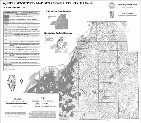
Figure 1. Aquifer Sensitivity Map of Tazewell County, Illinois, one of nine maps created for Tazewell County by the ISGS. Actual map was delivered at 1:62,500 scale in full color. |
Follmer, L.R., McKay, E.D., Lineback, J.A., and Gross, D.L., 1979, Wisconsin, Sangamonian, and Illinoian stratigraphy in central Illinois: Illinois State Geological Survey Guidebook 13, 139 p.
Hansel, A.K., and Johnson, W.H, 1996, Wedron and Mason Groups: lithostratigraphic reclassification of deposits of the Wisconsin Episode, Lake Michigan Lobe area: Illinois State Geological Survey Bulletin 104, 116 p.
Herzog, B.L., Wilson, S.D., Larson, D.R., Smith, E.C., Larson, T.H., and Greenslate, M.L., 1995, Hydrogeology and groundwater availability in southwest McLean and southwest Tazewell Counties, Part 1: Aquifer characterization: Illinois State Geological Survey and Illinois State Water Survey Cooperative Groundwater Report 17, 70 p.
Lineback, J.A., 1979, Quaternary deposits of Illinois: Illinois State Geological Survey, map, scale 1:500,000.
McGarry, C.S., and Grimley, D.A., 1997, Maps of Carroll County, Illinois: Illinois State Geological Survey Opne File Series 1997-13 a through k (11 maps), scale 1:62,500.
Riggs, M.H., McGarry, C.S., and Medlin, S., 2000, Maps of Jo Daviess County, Illinois: Illinois State Geological Survey Open File Series 2000-8 a through j (10 maps), scale 1:62,500.
Teater, W.M., 1996, Soil survey of Tazewell County, Illinois: U.S. Department of Agriculture, Natural Resources Conservation Service, 210 p. and maps.
Wilson, S.D., Kempton, J.P., and Lott, R.B., 1994, The Sankoty-Mahomet Aquifer in the confluence area of the Mackinaw and Mahomet Bedrock Valleys, central Illinois: Illinois State Water Survey and Illinois State Geological Survey Co-operative Groundwater Report 16, 64 p.