Digital Mapping Techniques '02 -- Workshop Proceedings
U.S. Geological Survey Open-File Report 02-370

Visualizing the Uncertainty of Geologic Maps

By Patrick J. Kennelly

Montana Bureau of Mines and Geology
Montana Tech of the University of Montana
Butte, MT 59701-8997
Telephone: (406) 496-2986
Fax: (406) 496-4451
e-mail: pkennelly@mtech.edu

ABSTRACT

INTRODUCTION

UNCERTAINTY OF TOPOGRAPHIC MAPS

To measure topographic uncertainty, the USGS generally uses 28 test points to determine the vertical accuracy of a 7.5-minute sheet. From these test points, a root mean square error (RMSE) can be calculated using the following equation:

where d_i = Z_estimated -Z_observed and n is the number of sample points. Given this RMSE, the USGS has assigned all DEM's to one of three categories. Level 1 DEM's are derived using photogrammetric techniques, and contain the least vertical error. They have a RMSE of 7 meters or less (Slocum, 1999).

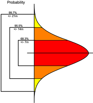
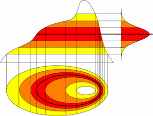
The RMSE is a summary statistic for a map. It gives no indication of how error is distributed, statistically or spatially. Error curves of very different shapes (e.g., normal, skewed) could have the same RMSE. Additionally, one segment of a map could account for the majority of the error in the map (Shortridge, 2001). In this study, I made the simplifying assumptions that (1) the error has a normal or Gaussian distribution (Figure 1), and (2) this error is distributed across the map.

Figure 1. A normal or Gaussian distribution curve. Values within one standard deviation account for 68.3% of the values and are shown in dark gray. Values within two standard deviations account for 95.5% of the values and include the medium-gray areas. Values within three standard deviations account for 99.7% of the values and include the light-gray areas.

LOCATION AND GEOLOGY OF THE STUDY AREA

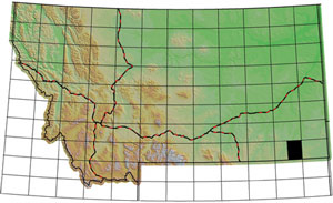
Figure 2. Location of the study area within the eastern half of the USGS Broadus, Montana, 30 x 60 minute quadrangle, southeastern Montana. The area is approximately 40 km by 55 km.

Geologic structure in this area is minimal and is characterized by low-angle bedding dipping to the northwest. The geologic contacts were constructed from a combination of field observations, regional correlations, and integration of previous mapping. In many cases contacts were interpolated between observed locations by the mapper, using knowledge of the structural orientation of the units and contours from the USGS topographic base maps.

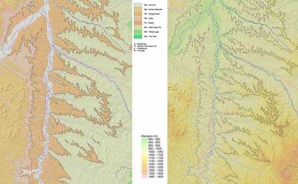
Figure 3. Geologic units of the eastern half of the USGS Broadus, Montana, 30 x 60 minute quadrangle.				Figure 4. Topography of the eastern half of the USGS Broadus 30 x 60 minute quadrangle, overlain with contacts of the geologic units from Figure 3.

The topography in the study area ranges from elevations of 900 to 1,350 meters (Figure 4). Slopes are as steep as 37°. The Little Powder River runs through the center of the study area, and associated Quaternary alluvium overlies the bedrock geology.

METHODOLOGY

A horizontal distance of 200, 400, and 600 meters was defined as the maximum horizontal width associated with the vertical buffers of ±7, 14, and 21 meters, respectively. This definition prevented inclusion of areas that are unrealistic distances from interpreted contacts based on the geologist's assesment. The gentle dip of geologic formations was ignored in this analysis. At the maximum horizontal distance of 600 meters from the contact, dips of 5° offset horizontal locations by approximately 50 meters.

RESULTS

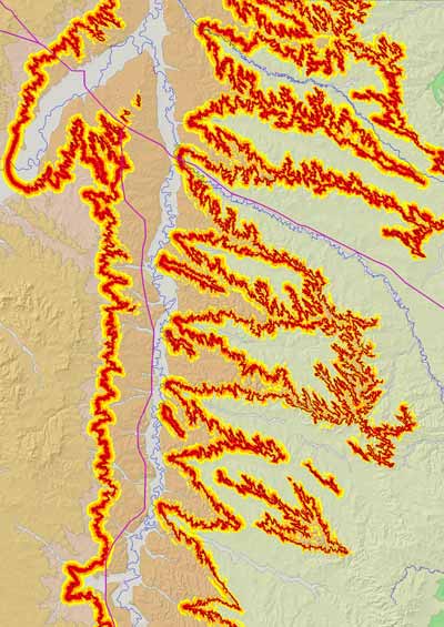
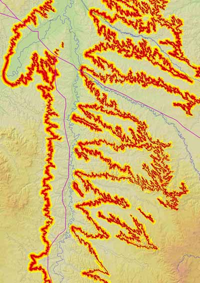
Figure 5. Probability of the geologic contact being within the dark-gray, medium-gray, and light-gray areas displayed on the geologic map; compare with Figure 1. The areas were defined using a vertical buffer.

Figure 6. Probability of the geologic contact being within the dark-gray, medium-gray, and light-gray areas displayed on the topographic map; compare with Figure 1. The areas were defined using a vertical buffer.

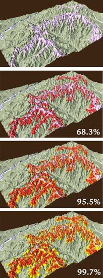
The horizontal width of the resulting buffer is highly variable. For the third standard deviation (dark gray, medium gray, and light gray), the width ranges from 90 to 1,200 meters (using the arbitrary maximum horizontal distance of 600 meters on each side of the contact). The width is greater in gently sloping areas and lesser in steeply sloping areas. The effect of slope on the probability of properly locating the contact in cross-sectional and map views is illustrated in Figure 7, and shown in perspective view for a part of the geologic map in Figure 8.

Figure 7. Normal distribution of error is shown on a cross-sectional view and map view of a sample location. Vertical widths are constant, but horizontal widths vary with the slope of the topography.

Figure 8. Perspective view of the east-central part of the geologic map from Figure 3. The Tullock Member overlies the Hell Creek Formation. Each frame adds a gray buffer to represent an additional standard deviation of locational error.

DISCUSSION

Alternatively, elevation values could be assigned to the top and basal contacts, and then a surface could be fit to the lines in three dimensions. A best-fit planar analysis in three dimensions would be equivalent to a linear regression of point data in two dimensions; then the surface could be offset by the RMSE z-values and intersected with the DEM. This method has two disadvantages. First, all segments of contact lines need not fall directly on the surfaces. Thus, there could be local variations not interpreted by the geologist. Second, new areas could be added in regions where the geologist has interpreted the contact as not present. In fact, the latter is the case in the southeastern corner of the study area. The Tertiary Tullock Member was determined to be absent on the basis of pollen samples, although the known topography and geologic structure would indicate that it should be present. The geologic interpretation is that structural dip increases in the southeastern part of the study area.

Areas inappropriate for this type of analysis include those where bedrock geologic contacts are overlain by alluvium. At these locales, the geologist has interpreted the location of the contact beneath the alluvium. Thus, the surface elevation, which now represents the top of the alluvium, is no longer appropriate. In areas where the contact is overlain by alluvium, such as in the stream valley in the northwestern part of the map, an evenly spaced concentric buffer pattern is apparent in Figure 5. The assumption that errors in elevation follow a normal curve is critical to the validity of this method. If error is random, the distribution should be normal (Wise, 1998). Systematic error, however, would not have a normal distribution. One such sampling error in the construction of DEM's is referred to as the "Firth Effect" and results in north-south or east-west lineations. This effect is caused by operators of photogrammetric equipment sampling row by row or column by column in alternating directions, and consistently underestimating elevation when moving upslope and overestimating elevation when moving downslope (Hunter and Goodchild, 1995). Visual inspection of hillshaded DEM's clearly reveal this striped pattern. These DEM's are generally not Level 1 and should be avoided for analysis.

CONCLUSIONS

This GIS method could be a reconnaissance tool used by geologists to determine the areas requiring more detailed field inspection. The method would be especially useful in larger scale mapping, such as 1:24,000 scale.

REFERENCES

Hunter, G.J., and Goodchild, M.F., 1995, Dealing with error in spatial databases: a simple case study: Photogrammetric Engineering and Remote Sensing, v. 61, p. 529Ð537.

Shortridge, A., 2001, Characterizing uncertainty in digital elevation models, in Hunsaker, C.T., Goodchild, M.F., Friedl, M.A., and Case, T.J., eds., Spatial uncertainty in ecology: implications for remote sensing and GIS applications: New York, Springer-Verlag, p. 238-257.

Slocum, T., 1999, Thematic cartography and visualization: Upper Saddle River, N. J: Prentice-Hall, Inc., 293 p.

U.S. Geological Survey, 2000, U.S. GeoData digital elevation models: U.S. Department of the Interior Fact Sheet 040-00: Washington, D.C., . U.S. Geological Survey, 1998, National Mapping Program technical instructions: standards for digital elevation models: U.S. Department of the Interior, .

Vuke, S.M., Heffern, E.L., Bergantino, R.N., and Colton, R.B., 2001, Geologic map of the Broadus 30- x 60-minute quadrangle, eastern Montana: Montana Bureau of Mines and Geology Open File Report #432, scale 1:100,000.

Wise, S.M., 1998, The effect of GIS interpolation errors on the use of digital elevation models in geomorphology, in Lane, S.N., Richards, K.S., and Chandler, J.H., eds., Landform monitoring, modeling and analysis: Chichester, England, John Wiley and Sons, p. 139-164.