Ohio Geological Survey
4383 Fountain Square Drive
Columbus, OH 43224
Telephone: (614) 265-6601
Fax: (614) 447-1918
e-mail: jim.mcdonald@dnr.state.oh.us
Computer-based technology was used to expedite completion of the reconnaissance-bedrock-geology mapping through digital generation of structure-contour maps of the units mapped. Computer techniques were developed to minimize edge effects during the gridding and contouring process. Other techniques were developed to assist in edge-matching of the maps produced by the geologists. Final output of the structure-contour maps was edited using CAD software that interfaced with the gridding and contouring software. The computer mapping software enabled the ODGS to complete the reconnaissance remapping of the bedrock geology of the state in the relatively short time period of seven years.
The 1920 state bedrock-geology map was inaccurate in many areas, used outdated stratigraphic nomenclature, was highly generalized, and was plotted on a now-outdated, 1:500,000-scale base map. Between 1918 and 1979, there were numerous changes in stratigraphic nomenclature and concepts, some of which dated the older style of mapping. For example, starting in the mid-1950's, the Survey began using lithostratigraphic units to describe formations, instead of chronolithostratigraphic terminology. In addition, there have been advances in the understanding of the bedrock topography of the state. While standard topographic maps can be used to depict bedrock contacts in the nondrift-covered areas, bedrock-topography maps are required to delineate the bedrock geology across the glaciated portion of the state, which covers two-thirds of the state. Finally, new planimetric and topographic base maps have been made for Ohio by the U.S. Geological Survey, which allow the ODGS to more accurately depict the bedrock geology and cultural features in the state.
Mapping of the bedrock geology has been ongoing since the release of the 1920 bedrock geology map. From 1918 to 1979, the ODGS conducted county-level geologic mapping at the scales of 1:62,500 and smaller, on base maps constructed from the U.S. Geological Survey 15-minute-topographic quadrangles (Sherman, 1933). Only 18 counties had been completed by the time the last county bulletin was published in 1977 (Collins and Smith, 1977). Starting in the late 1960's, a more detailed level of mapping was initiated. Between 1957 and 1963, a new topographic map series was created at a scale of 1:24,000 by the U.S. Geological Survey (Bernhagen, 1994). With the completion of that program, there were a number of initiatives, starting in the mid-1960's (DeLong, 1965), to perform detailed geologic mapping at the 1:24,000 scale. By the end of the 1980's, only 37 quadrangles, out of 788, had been completed, and it became apparent that the new detailed bedrock-geology mapping effort was going to take over 100 years to cover the entire state. With the appointment of a new state geologist in 1989, a new program was initiated at the ODGS to perform more rapid reconnaissance geologic mapping at 1:24,000 scale, using supplemental funds from U.S. Geological Survey STATEMAP grants, U.S. EPA Nonpoint-Source Pollution 319-A funds, and ODOT grants. This program would allow the completion of a new statewide geologic map in a few years.
In order to complete mapping in such a short period, the use of computer mapping software was necessary. The software would be used to create structure-contour maps of the units being mapped and would accelerate the mapping in a number of ways. The software would reside on individual geologists' PC's, thereby allowing the geologists' easy access to the software and structure-contour maps at any time. The software would be programmed to minimize the problem of edge-matching within, and outside, the geologist's project area. Finally, multiple versions of the structure-contour maps could be created very easily, thereby allowing the geologist to easily correct problems and test multiple hypotheses. This paper describes the gridding algorithm and mapping technique used to automate the creation of structure-contour maps for the statewide mapping of the bedrock geology in Ohio.
|
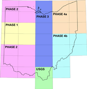
Figure 1. Map showing the different phases of the bedrock-geology mapping program. |
|
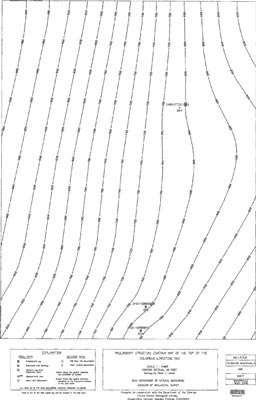
Figure 2. A computer-generated structure-contour map, as released in the ODGS informal, open-file series.
VIEW a printable PDF file in a new window. |
Structure-contour maps were then used in conjunction with bedrock-topography and surface-hypsography maps to produce 1:24,000-scale bedrock-geology maps. The structure-contour maps were overlain with bedrock-topography maps and surface hypsography. At the location where the structure-contour elevation intersected the surface hypsography or the bedrock topography, the unit contact was drawn (Figure 3). Depending on how many units were present in the area at the surface or subcrop, between one and eight different structure-contour maps were drawn per 7.5-minute quadrangle. By the end of the project, the geologists had created more than 1,840 structure-contour maps for the bedrock-geology mapping project. It was only through the use of the computer-mapping software that such a large number of maps could be created in such a short period of time.
|
Figure 3. An open-file structure-contour map is overlain with the bedrock-topography map and surface hypsography. Where the structure-contour surface intersects the bedrock-topography surface, bedrock contacts are drawn. In this example, the solid lines are the structure contours, the dashed lines are the bedrock-topography contours, and the dotted line is the bedrock contact. |
On the basis of its own experience and upon discussions with the technical staff at the Radian Corporation, ODGS decided to use a proprietary gridding algorithm created by the Radian Corporation called convergent gridding (Haecker, 1992). This algorithm appeared to minimize the edge effects that are produced by other gridding algorithms, such as minimum curvature or least squares. When gridding parameters are properly set up, the gridding algorithm also would honor the data points. These aspects of minimizing the edge effects and honoring the data points greatly attracted ODGS to use the convergent gridding algorithm.
Other types of gridding algorithms, such as least squares or minimum curvature, produce a number of undesirable effects when creating a grid of calculated values from the original data. One of the undesirable effects is that most gridding algorithms do not honor the original data points. These algorithms may produce a grid of calculated values that conflict with the original data values. Another undesirable effect is edge effects. Most algorithms compute the first and second derivatives (slope and curvature) during the process of creating the grid. At the edge of the gridding area, critical information is not available and the derivatives cannot be correctly computed. Most software programs make assumptions about the first and second derivatives at the edge of the gridding area. The surfaces that they produce generally are wildly divergent from what is expected. The convergent gridding algorithm used in the CPS/PC program minimized these edge effects, but, as was discovered during the project, the algorithm did not totally remove them from the resulting calculated grid. For ODGS to further minimize the edge effects from the maps, ODGS implemented a number of different data-handling and processing techniques, described in a later section.
The convergent gridding algorithm was developed by the Radian Corporation to help honor the original data points and to help minimize the edge effects (Haecker, 1992). The first step in computing the grid is to assign the values of the data points to the initial grid that was set up as part of the gridding parameters. The initial grid values comprise the data point values, the slope, and the curvature of the nearest grid values. Each grid node undergoes a smoothing process using a biharmonic Taylor series. The next step is to divide the grid in half, in the X and Y directions. The data points and the previous grid-node values are then assigned to the nearest grid nodes. The biharmonic smoothing process is then applied again to the grid-node values. The process continues until the final grid-node-spacing value is reached. Also, at any point, additional data can be introduced during the gridding process. Once the gridding algorithm converges on a solution, contouring can begin (Haecker, 1992).
For the final maps at 1:24,000 scale, the geologist used a final grid interval of 2,000 feet in the X and Y directions. This grid interval was generally small enough to ensure that every data point would be honored by the structure contours. Once the final grid for each structure-contour map was created, a macro routine was used to cut out the grid nodes within a 7.5-minute quadrangle area, from either the 1° x 2° block (Phase 1) or from the 30 x 60 minute quadrangles (Phases 2 through 4b). In order for contouring to extend to the boundary of the quadrangle, the grid nodes up to 2,000 feet away from the quadrangle boundary also were cut out during the process. After contouring was completed, the contours were cut off at the quadrangle boundaries to create a publication-quality map.
The first two techniques, the use of data points outside of the mapping area and gridding outside the mapping area, used in conjunction with one another are well known in the mitigation of edge effects (Davis, 1986). Figures 4 and 5 show an example of the two techniques for the Marion 30 x 60 minute quadrangle and the 32 7.5-minute quadrangles within it. In the first technique, data points both within and outside the mapping area are used in the gridding process (Figure 4). The data points outside the mapping area provide control up to the edge of the area to be mapped. The second technique, gridding outside of the mapping area, is shown in Figure 5. Figure 5a shows what happens when gridding occurs up to the boundary of the intended mapping area. Typically, geologists using mapping software will create a grid only within the intended mapping area to allow the contours to stop at the boundary of the mapping area. Unfortunately, this method produces edge effects within the intended mapping area. By expanding the gridding area beyond the mapping area, the edge effects are moved outside the mapping area. In Figure 5b, the gridding was expanded out by one row of 7.5-minute quadrangles. By expanding the gridded area, the edge effects are moved away from the intended mapping area.
|
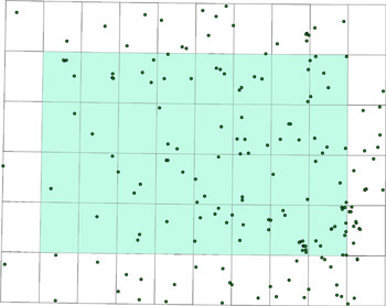
Figure 4. Example of a mapping area and the data points used to create the structure-contour map. The structure-contour map is created using data from both inside and outside the mapping area. This pulls the edge effects away from the project area. In this figure, the mapping area is the Marion 30 x 60 minute quadrangle. |
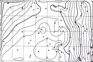
Figure 5a. Example of a grid area that is the same size as the mapping area. In this example of the Marion 30 x 60 minute quadrangle, the edge effects are most noticeable on the western boundary. Edge effects are less noticeable on the northern and southern boundaries. Because there is a well-pronounced dip into the Appalachian Basin on the eastern boundary of the Marion 30 x 60 minute quadrangle, the edge effects here are not noticeable. |
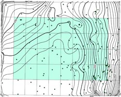
Figure 5b. Example of a grid that is larger than the mapping area. Edge effects are minimized because they are located outside the actual mapping area. |
The next technique is the use of pseudodata points along and outside of the outcrop line. Serious edge-effect problems occur when the subsurface structure-contour mapping approaches the surface outcrop line. Because the unit being mapped does not exist beyond the outcrop, there is no way to control the subsurface structure-contour mapping close to the outcrop. The use of pseudodata points near the outcrop can minimize contouring errors by providing additional control for the mapping software (Figure 6). An elevation is supplied to the pseudodata point by a number of methods. If there is sufficient outcrop exposure, the geologist may assign an elevation to the point based upon the nearby outcrop elevation. Otherwise, an elevation is assigned to the pseudodata point using a preliminary structure-contour map. Projections are made out into space, to the pseudodata point, using the preliminary computer-generated structure-contour map. The elevations of the pseudodata points are then adjusted upward or downward on the basis of a structure-contour map of an underlying unit and an isopach map of the unit being mapped. The modified pseudodata points are then included in the database and a second round of computer mapping is performed. Iterations of this technique continue until an acceptable structure-contour map is created.
|
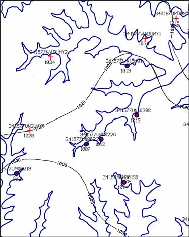
Figure 6. In this example, pseudodata points and data points are used to help create the structure-contour map. The light solid lines are the structure contours, the heavier solid line is the bedrock contact, the solid-filled circles represent the data points, and the crosses represent the pseudodata points. |
In some cases, using data and grid nodes from two 1:24,000-scale quadrangles beyond the project areas were not enough to remove edge effects. In addition, the geologists did not always use the surrounding grid nodes as part of their gridding process. In either case, the contours did not match the previously created structure-contour maps. If that was the case, after the 1:24,000-scale structure-contour map was created, the geologist would edge-match the structure-contour maps by hand. While there were always instances where edge-matching between different mapping areas was done by hand, the techniques described above helped minimize the amount of edge-matching that had to be done during this program.
One of the most serious problems with using computer gridding and contouring software is that the software algorithms produce edge effects. The gridding algorithm used for this project, when assisted by the techniques described in this paper, tended to minimize the edge effects.
Techniques also were created to perform edge-matching using the computer. These techniques allowed for the individual project map areas to be merged together somewhat seamlessly, in addition to minimizing the amount of edge-matching along the border of the mapping areas. These techniques were generally successful, but edge-matching between the project areas by hand (in CAD) still had to be performed. While this was an inconvenience, the use of the computer to perform the contouring routines eliminated the need for edge-matching among the 1:24,000-scale maps within each project area and greatly sped up the mapping process.
The use of computer gridding and contouring allowed for multiple maps to be made quickly, seamlessly, without edge effects, and plotted in a professional-looking output. The geologists could generate multiple hypotheses and see which one allowed for the best geologic interpretation. If the parameters that were selected did not produce a geologically realistic structure-contour map, then other parameters could be selected rather easily.
Bownocker, J.A., 1920, Geologic map of Ohio: Ohio Division of Geological Survey Map 1, scale 1:500,000, 1 sheet.
Collins, H.R., and Smith, B.R., 1977, Geology and mineral resources of Washington County, Ohio: Ohio Division of Geological Survey Bulletin 66, 134 p.
Davis, J.C., 1986, Statistics and data analysis in geology (2nd ed.): John Wiley & Sons, 686 p.
DeLong, R.M., 1965, Geology of the Kensington quadrangle, Ohio: Ohio Division of Geological Survey Report of Investigations 55, scale 1:24,000, 1 sheet.
Haecker, M.A., 1992, Convergent gridding: a new approach to surface reconstruction: Geobyte, v. 7, no. 3, p. 48-53.
Sherman, C.E., 1933, Miscellaneous data: Ohio Cooperative Topographic Survey, Volume IV of the Final Report, 327 p.