Digital Mapping Techniques '03 — Workshop Proceedings
U.S. Geological Survey Open-File Report 03–471

Alaska Digital Mapping Project: From Field to Publication

By Christopher P. Garrity

U.S. Geological Survey, National Center, MS 956, 12201 Sunrise Valley Drive, Reston, VA 20192
Telephone (703) 648-6426; fax: (703) 648-6419; e-mail cgarrity@usgs.gov

INTRODUCTION

The natural resources of northern Alaska continue to be a focus of national attention. As a result, the need for detailed geologic maps is greater than ever, not only as a basis for petroleum and mineral exploration, but also for land-use planning and mitigation of environmental impacts. The U.S. Geological Survey (USGS), in cooperation with the Alaska Division of Oil and Gas, has embarked on a project to map the northern front and foothills of the Brooks Range of northern Alaska. The goal of the project is to publish an integrated set of digital geologic maps with consistent stratigraphic nomenclature and a standardized cartographic style. Initial field work in the Alaska North Slope, including the northern front and foothills of the Brooks Range, was accomplished between 1944 and 1953 by the USGS. Maps stemming from that work were published between 1957 and 1966 as USGS Professional Papers 303 A—H. Since then, numerous geologic maps of individual quadrangles at various scales have been published by the USGS and by the Alaska Division of Geological and Geophysical Surveys. These maps provide a broad framework of the stratigraphy and general outcrop distribution of northern Alaska. The current project builds from these maps, incorporating new field observations, modern stratigraphic terminology, and contemporary digital mapping techniques (for example, Mull, 2003).

This paper discusses techniques employed in digitally capturing the geologic maps of northern Alaska and the post-capture procedures used in preparing publications. A variety of Geographical Information Systems (GIS) and graphical software applications, including ArcGIS, Adobe Illustrator, Adobe Photoshop, and Avenza MAPublisher were used in the cartographic production process.

IMAGE CAPTURE AND PREPARATION

For this project, original geologic linework and subsequent map revisions were drafted on stable-base mylar, which substantially reduced the swelling, shrinking, and folding errors commonly associated with scanning paper maps. Before stable-base mylars were scanned, the scanner was serviced to assure proper camera alignment and roller control. Mylars were then scanned at a resolution of 400 dots per inch (dpi) and saved as an 8-bit grayscale Tagged Image File Format (TIFF) image. The improved clarity gained by scanning at a resolution greater than 400 dpi did not merit the resulting increase in file size.

Post-scan image filtering was done in Adobe Photoshop. The first filter applied to grayscale TIFF images was “unsharpen mask.” This filter identified contrast edges in the image and increased the overall contrast, which performed exceptionally well in defining geologic contact lines. The “amount” was set to 200%, with a radius of about 1.5 pixels and a threshold level of 0%. Applying the filter lessened the amount of image “wash-out” when the grayscale image was later converted to monochrome. The next step, easily the most time-consuming part of the digital capturing process, was to remove the non-essential elements in the image (geologic unit labels, strike and dip symbols, leaders, etc.). Eraser tools in Adobe Photoshop and raster-cleanup tools in ArcScan were used for this. Finally, the image was converted from 8-bit grayscale to 1-bit monochrome, using the 50% threshold option (fig.1). This option converted pixels with gray values above the middle gray level (value=128) to white and converted gray levels below the middle level to black. A thorough visual analysis of the image was performed to ensure that features were not washedout upon conversion. Conversion to monochrome was useful, as ArcScan requires images to be bi-level (two unique colors) prior to vectorization. An additional benefit associated with the monochrome conversion was a significant reduction in file size.

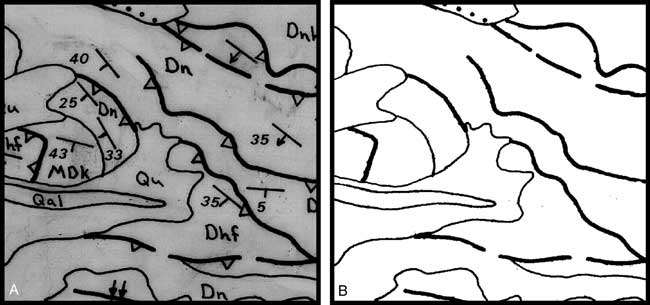Figure 1. Preparing images for autovectorization. (A) Original grayscale image scanned at 400 dpi. (B) Monochrome image after unwanted raster elements were removed.

The final step before vectorization was to georeference the image using the georeference tools in ArcMap. The image was georeferenced by adding Universal Transverse Mercator (UTM) coordinates to each latitude and longitude tick-mark on the source map. After an acceptable Root Mean Square error value was attained, the image was rectified and added to the data frame.

STABLE-BASE VECTORIZATION

TIFF images were autovectorized using the ArcScan extension in ArcGIS 8.3. Almost all raster-to-vector conversions were accomplished through batch (automated) vectorization. This method was less time-consuming than interactive vectorization, although sections of numerous maps were nevertheless vectorized interactively. Problem areas encountered in the batch vectorization process were repaired with the suite of raster painting tools available in the raster painting toolbar (fig. 2).

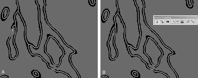Figure 2. Raster cleanup in ArcScan. (A) A section of the raster image (black pixels) failed to be detected by the scanner. (B) The section was repaired with the raster painting brush, and the vector preview (white pixels) was generated interactively.

The geometry of the resulting vector data was controlled in the vectorization settings menu. To maintain the integrity of the source linework, special attention was paid when adjusting settings. All maps were vectorized using the centerline vectorization method. Vectorization settings used for digital capture of source scans included the following:

• Intersection solution was set to median; median is designed for nonrectilinear intersections (ideal for geologic maps).
• Maximum line-width setting varied by scan, but was used to extract vectors representing the same feature in the source map (for example, faults or geologic contacts).
• Compression tolerance was set between 0.005 and 0.050, depending on the complexity of the source map. This produced smooth vectors and represented the source linework accurately. When figures with angular intersections were vectorized, compression tolerance was increased significantly to generate straight-line vectors with a limited number of vertices.
• Smoothing weight was set between 1 and 3. When levels were set higher than 3, misinterpretation of the source data commonly occurred.
• Gap closure tolerance was used when inferred or concealed line symbols were denoted in the source map. When the setting was activated, vectors would sometimes connect to random speckles in the image, generating unwanted line features. For this reason, all source images were despeckled before vectorization.

By using the maximum line width setting and raster-cell selection tools, vector data representing the same feature were extracted and saved into separate data layers. This proved to be helpful when vector data were attributed. Separate data layers were saved in ArcInfo coverage format and integrated into the digital database. Finally, ArcInfo export files were generated for cartographic production in Adobe Illustrator via MAPublisher.

FILM POSITIVE BASES

For each quadrangle, topography, drainage, and open-water film positives for base-map compilation were ordered through the USGS Eastern Publications group. Unfortunately, open-water separates were not available for every quadrangle, and in some instances had to be generated by autovectorizing drainage positives. In these cases, the same scanning procedures discussed above were applied. After polygon topology was built, open-water polygons were extracted and saved as a new coverage. For all other separates, scanner threshold settings were adjusted and film positives were scanned directly to monochrome. A monochrome output was chosen because all background pixels (white fill areas) appear transparent when opened in Adobe Illustrator. Base map layers could then be placed over other graphic layers without concealing them. Positives were scanned at a resolution of 600 dpi to avoid legibility problems in areas where linework was very fine. Image collar information was trimmed and speckles were removed before being georeferenced in ArcMap. Georeferenced images were positioned accurately relative to underlying vector geology using the MAPublisher register image filter. Base images were placed as links in Illustrator so that future image editing could be accomplished “on the fly.” Color choices for base-map separates were as follows:

• A 50–65% gray level was applied to the topography/culture separate. Gray levels were adjusted on the basis of the complexity of the raster image. When levels above 65% were applied, the raster image began to obscure underlying vector data and was generally too overbearing. When gray levels below 50% were applied, the raster image suffered from diminished legibility in areas where underlying colors were light.
• A 100% cyan level was applied to the drainage separate. This distinguished the drainage separate from the open-water separate, which was assigned a cyan level near 25%. In areas where underlying layers had a high cyan content, image color levels were adjusted to avoid legibility problems.

CARTOGRAPHIC DESIGN

ArcInfo export files were imported into Adobe Illustrator via MAPublisher for cartographic production. In some cases, arcs with too many vertices created diced polygons upon import (fig. 3). Although setting the grain tolerance in MAPublisher can resolve this dilemma, in areas where problems remained, arcs were generalized in ArcInfo. After coverages were imported, all unique features were released into separate layers for greater ease in editing and review. By importing via MAPublisher, attributes were retained, allowing unique features to be selected with the “select by attribute” feature. This was quite helpful when stroking line features, using USGS digital cartographic standards (U.S. Geological Survey, 2000). Federal Geographic Data Committee (FGDC) compliant cartographic specifications in PostScript format were easily implemented in Adobe Illustrator with the eyedropper tool. Line features requiring uniform symbols along their axes ( thrust fault teeth, hachure marks, etc.) were built as pattern brushes in Adobe Illustrator to ensure accurate symbol placement without the need to place symbols individually. Point features requiring rotation, such as strike and dip, were rotated in ArcGIS via a rotation field and exported in PostScript format. Collar text information, including correlation of map units, description of map units, discussion, and references, was pasted into text boxes for ease in standardization. Finally, drafts were sent to the USGS Eastern Publications Group for technical review and editing.

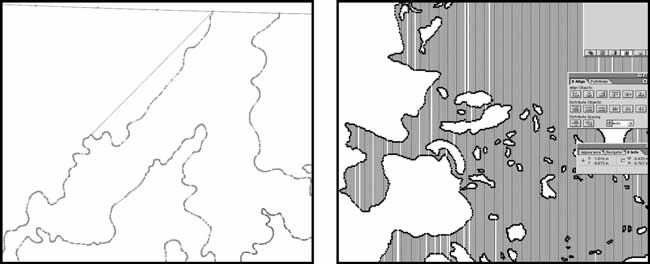Figure 3. Two examples of diced polygons in MAPublisher. This occurs when arcs have too many vertices, and is easily resolved by generalizing problem arcs in ArcInfo.

Completed digital quadrangles have been converted to Printable Document Format (PDF) files for future online release. Ultimately, through the World Wide Web, users will be able to download the PDF files, ArcInfo coverages, or order hard copies through the map-on-demand process. Plotting-on-demand eliminates the need to make expensive color-separated negatives, but generally does not meet the same quality and accuracy standards as lithographically printed products.

REFERENCES

Mull, C.G, Houseknecht, D.W., and Bird, K.J., 2003, Revised Cretaceous and Tertiary stratigraphic nomenclature in the Colville Basin, northern Alaska: U.S. Geological Survey Professional Paper 1673, 59 p.,http://pubs.usgs.gov/pp/p1673/.

Mull, C.G, Houseknecht, D.W., and Pessel, G. H., in press-2003, Geologic map of the Umiat quadrangle, Alaska: U.S. Geological Survey MF map, scale 1:250,000.

U.S. Geological Survey, 2000, Public Review Draft–Digital cartographic standards for geologic map information: U.S. Geological Survey Open-File Report 99-430, p. 1-18, http://geopubs.wr .usgs.gov/open-file/of99-430/.