Digital Mapping Techniques '03 — Workshop Proceedings
U.S. Geological Survey Open-File Report 03–471

Bedrock Geology and Bedrock Topography GIS of Ohio: New Data and Applications for Public Access

By James McDonald, E. Mac Swinford, Lawrence H. Wickstrom, Ernie R. Slucher, Donovan M. Powers, and Thomas M. Berg

Ohio Division of Geological Survey, 4383 Fountain Square Drive, Columbus, OH 43224
Telephone (614) 265-6601; fax (614) 447-1918; e-mail jim.mcdonald@dnr.state.oh.us, mac.swinford@dnr.state.oh.us, larry.wickstrom@dnr.state.oh.us, ernie.slucher@dnr.state.oh.us, donovan.powers@dnr.state.oh.us, thomas.berg@dnr.state.oh.us

INTRODUCTION

The Ohio Division of Geological Survey (ODGS) recently completed four major geographic information systems (GIS) data sets: bedrock geology and bedrock topography at 1:24,000 scale, and bedrock geology and bedrock topography at 1:500,000 scale. These data sets, the result of several geologic mapping cooperative programs between ODGS and various state and federal agencies, represent a major advance for the ODGS and its goal of providing digital geologic information for the general public.

This summary briefly describes the history and procedures used to map the bedrock geology and bedrock topography of Ohio and the conversion of the open-file 1:24,000-scale bedrock geology and bedrock topography maps into GIS data layers. The 1:24,000-scale bedrock geology and bedrock topography data sets form the framework for the new 1:500,000-scale bedrock geology and bedrock topography maps and GIS data layers. In addition, computer applications were developed to plot the maps and export GIS data layers for individual 7.5-minute quadrangles. These applications will allow the ODGS to manage and update the GIS data sets and will assist in the distribution of the maps and GIS data sets to the public.

GEOLOGIC MAPPING IN OHIO

Prior to the completion of the new bedrock geology maps and GIS data sets, Ohio’s 1920-vintage state bedrock geology map was one of the oldest in-print state bedrock geology maps in the nation (Bownocker, 1920). Mapping of Ohio’s bedrock geology has been going on since the release of the 1920 map, but had not resulted in the production of a new statewide bedrock geology map. From 1918 to 1979, the ODGS conducted geologic mapping on the county level at scales of 1:62,500 and smaller, on base maps constructed from the U.S. Geological Survey (USGS) 15-minute topographic quadrangles (Sherman, 1933). Only 19 of the 88 counties had been completed by the time the last county report (Cuyahoga County) was published (Ford, 1987). Starting in the late 1960s, a more detailed level of mapping was initiated. Between 1957 and 1963, a new topographic map series was created for Ohio at a scale of 1:24,000 by the USGS (Bernhagen, 1994). With the completion of that program, there were a number of initiatives, starting in the mid-1960s (e.g. DeLong, 1965), to perform detailed, field-based geologic mapping at 1:24,000 scale. By the end of the 1980s, only 37 quadrangles, out of 788, had been completed and it became apparent that, with the current staffing level, completing the new detailed bedrock geology mapping effort for the entire state would take more than 100 years.

With the appointment of a new state geologist in 1989, a program was initiated at the ODGS to perform more rapid reconnaissance-level geologic mapping at 1:24,000 scale, funded by a portion of the Ohio Minerals Severance Tax and supplemented by funds from USGS COGEOMAP and STATEMAP grants, U.S. Environmental Protection Agency (EPA) Nonpoint-Source Pollution Program 319(h) grants, and grants from the Ohio Department of Transportation (ODOT). The reconnaissance approach to bedrock geology mapping relies less on detailed, field-based procedures and more on in-house data and analysis. The reconnaissance-mode techniques included limiting the stratigraphic resolution of the mapped units, the use of data that was collected over the last 120 years and stored in the ODGS archives, the use of existing bedrock topography maps, and the use of computers to assist in the mapping. These techniques, while admittedly reducing the possible detail, enabled the entire state to be mapped in 7 years, a fairly remarkable timeframe for such a large project (Swinford, 1997; McDonald, 2002).

Several methods were used to limit the stratigraphic resolution of the reconnaissance-level bedrock geology maps. For some stratigraphic intervals, mapping units were combined. For example, the Silurian Peebles Dolomite, Lilly Formation, and Bisher Formation were too thin to be mapped as individual units at 1:500,000 scale. These formations were combined to form a single unit—Peebles Dolomite, Lilly Formation, and Bisher Formation undivided. Some stratigraphic intervals, such as the Ordovician undifferentiated and the Mississippian undifferentiated, were not formally defined. In the case of the Ordovician undifferentiated, the physical characteristics and spatial variability of this lithologic unit, buried beneath glacial deposits, were too poorly understood to be formally defined. In another example, the Pottsville, Allegheny, Conemaugh, and Monongahela Groups of the Pennsylvanian System and the Dunkard Group of the Pennsylvanian-Permian Systems were not subdivided below the group level, in part because few of the internal units have any lateral continuity (Larsen, 1991). As a final example, individual coal beds were not mapped, except where they were used as key beds to define group boundaries. While each of these methods reduced the stratigraphic resolution of the mapping units, the process also decreased the amount of time needed to resolve stratigraphic problems and helped expedite the mapping.

There was a limited amount of fieldwork performed for this project. The data, some of which dated back 120 years, primarily came from the extensive ODGS archives. The data collection in the ODGS archives contains in excess of 17,000 measured stratigraphic sections, 4,000 core descriptions, 250,000 oil- and gas-well records, and many geologists’ field notebooks. Most of the measured stratigraphic section and core descriptions have been entered into the USGS’s National Coal Resources Data System (NCRDS). These NCRDS data points, together with the oil- and gas-well geophysical logs, were used to build cross sections and to identify the tops of mappable units in the subsurface. Where necessary, field work was performed to collect additional data to fill gaps and to resolve complex stratigraphic and structural issues. Eleven stratigraphic test core holes were drilled in western Ohio by ODGS to supplement areas of sparse data. These core holes were geophysically logged to allow correlation to nearby oil and gas wells.

Because nearly three-quarters of Ohio is covered by glacial and related deposits, the bedrock topography had to be mapped before the bedrock geology. The bedrock topography data set was created using many different sources. There has been an ongoing effort to map the bedrock topography since the early 1970s. At that time, the ODGS started mapping the bedrock topography on a county-by-county basis at 1:62,500 scale. In the mid-to-late 1980s, the ODGS began more detailed bedrock topography mapping on 7.5-minute quadrangles at 1:24,000 scale. In both instances, the bedrock topography was mapped using available water-well logs from the Ohio Division of Water, ODOT boring logs, and other data sources. For the reconnaissance bedrock geology mapping, the existing 1:62,500-scale county maps were photographically enlarged to 1:24,000 scale. In areas where there were no bedrock topography maps, new maps were created at 1:24,000-scale (figure 1).

Figure 1. A bedrock topography contour map of the Bellevue, Ohio 7.5-minute quadrangle, as released in the ODGS informal, open-file series.

The ODGS had just begun to use computers in the mid-to-late 1980s. In order to accelerate the pace of mapping, the ODGS in 1991 acquired PC-based gridding and contouring software to create structure contour maps of the mappable units in each quadrangle. Depending on how many contacts were present in the area at the surface or beneath the glacial drift, between one and eight different structure contour maps were drawn per 7.5-minute quadrangle (figure 2) (McDonald, 2002).

Figure 2. A computer-generated structure contour map, as released in the ODGS informal, open-file series. This is a structure contour map on the top of the Devonian Columbus Limestone of the Bellevue, Ohio 7.5-minute quadrangle.

Structure contour maps were used in conjunction with bedrock topography maps, drawn on USGS 7.5-minute topographic maps, to produce 1:24,000-scale bedrock geology maps. The structure contour maps were overlaid on hand-drawn bedrock topography maps which, in turn, were overlain by mylar 1:24,000-scale base maps. Bedrock contacts were drawn on the base maps where the structure contour surface intersected equivalent elevations on the bedrock topography or the surface topography maps, producing new bedrock geology maps (figure 3). By the end of the project, the geologists had created over 1,840 structure contour maps, 788 bedrock topography maps, and 788 bedrock geology maps (McDonald, 2002).

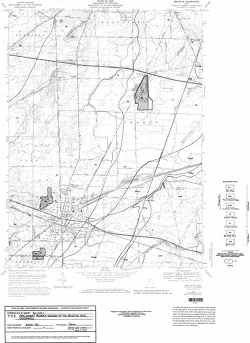Figure 3. A bedrock geology map of the Bellevue, Ohio 7.5-minute quadrangle, as released in the ODGS informal, open-file series.

1:24,000-SCALE BEDROCK GEOLOGY AND BEDROCK TOPOGRAPHY GIS

After the bedrock geology maps were drawn, the maps were converted to a GIS. Funding for GIS conversion came from the State of Ohio General Revenue Fund, supplemented by grants from ODOT and a USGS STATEMAP grant. The conversion was also abetted by two other factors. During the mid-1990s, the Ohio Office of Budget and Management allowed the use of capital funds, which are normally used for building and maintaining roads and buildings, for building digital data infrastructure elements. These elements included the conversion of data to a GIS, using outside contractors to perform the conversion.

The second factor was the initiation of a CAD/GIS conversion shop by the Ohio Penal Industries (Wickstrom, McDonald, and Berg, 1998). Using inmates trained in CAD and GIS software as a labor force, and private-sector contractors as project management, Ohio Penal Industries provided map digitizing services at a reasonable cost. ODGS was pleased by the quality of work provided by the inmates, who were motivated and took pride in the products they created. The work afforded them an opportunity to acquire meaningful training in the use of computers and software. Non-tangible incentives for the prison inmates assisted in keeping job satisfaction and quality of the GIS product at a high level.

The conversion of the bedrock geology and bedrock topography maps was performed over a 10-year period. Initially, ODGS staff digitized the bedrock geology maps of western and part of southern Ohio between 1992 and 1998. The ODGS staff and interns digitized the bedrock geology maps of the central part of the state under a USGS grant in 1996. Finally, the Ohio Penal Industries digitized the bedrock geology maps of the eastern part of the state in 1998 (figure 4). The ODGS staff digitized the bedrock topography maps for northwestern Ohio in 1992 and the central part of the state in 1996. The Ohio Penal Industries digitized the remaining bedrock topography maps, in southwestern and eastern Ohio, in 2001-2002.

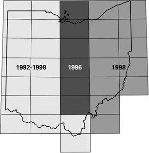Figure 4. Index map showing the years during which the bedrock geology maps were digitized.

Digitization of bedrock geology and bedrock topography data sets was accomplished using digitizing tables and heads-up digitizing techniques. ODGS staff and interns digitized the 7.5-minute quadrangle maps on a digitizing table, registering the map to a digital file containing the 7.5-minute quadrangle boundaries. The staff and interns then digitized the contact lines into the bedrock geology and bedrock topography CAD files. The inmates performed their work differently, first scanning the mylar maps and then registering the images to the correct quadrangle coordinates. They then did heads-up digitizing of the 7.5-minute quadrangle bedrock geology and bedrock topography maps.

The private-sector contractors provided project management and software programming, as well as training, guidance, and quality control for the inmates. The final project-management contractor also converted the CAD files to seamless ArcInfo coverages. The GIS files were then sent to ODGS for final quality control and acceptance, and were inspected by an ODGS college intern to ensure that the graphics and the polygon and line attributes were correctly captured. The GIS conversion was completed in 2002.

GENERALIZED BEDROCK GEOLOGY AND BEDROCK TOPOGRAPHY GIS

The new full color 1:500,000-scale state bedrock geology map (figure 5) was produced from geologic contacts compiled, generalized, and originally drawn at 1:250,000 scale. First, digital CAD files of edge-matched 7.5-minute (1:24,000) bedrock geology quadrangle maps were plotted onto mylar as 1:250,000-scale, 1 × 2-degree quadrangles. These were then overlaid by a second sheet of mylar containing reverse plots of the digital state transportation network (provided by ODOT) and a modified version of the digital drainage network (USGS). This second sheet of mylar served as the base map for all compilations.

Figure 5. A view of the new state bedrock geology map, to be published at 1:500,000 scale.

Printing these base map elements as reverse features (upside down and backwards) on the back side or bottom of two-sided mylar served two functions. First, although these plots would be on the back side of the mylar, they would appear geographically correct when placed right-side-up on a light table. Second, the top side of this same sheet of mylar could then serve as the drawing surface for the geologic contact phase of map compilation. This method was used so that any drawing errors made during the compilation phase could be corrected without destroying the transportation and drainage network features plotted on the back side of the base map.

Finally, all contact lines between mapped geologic units were duplicated and some were modified locally by hand. Generalizing and modification of these lines also assured that the hand drawn contact lines maintained their proper spatial relationships to the hydrology and transportation network elements on the map.

The generalized 1:250,000-scale contact lines were then scanned, registered to the new digital state transportation map, heads-up digitized into a CAD file, and converted to an ArcInfo coverage. Topology was created for these elements, with a fuzzy tolerance appropriate for a 1:250,000-scale map. Labels within the coverage area were attributed with the correct geologic unit abbreviation; individual (1 × 2-degree sheets) coverage areas were merged; and to finish the process, the boundaries between the individual map sheets were dissolved.

The generalized bedrock geology data set is composed of four separate GIS data layers. The geologic-unit polygons and contact lines are the two largest GIS data layers. The other two data layers contain structural elements (faults) and pinch-out lines. The term pinch-out lines is a special connotation developed during the project to designate those areas on the map where, because of high topographic relief or lithologic thinning of a geologic unit, two adjacent geologic contact lines between different map units were merged together to form a single line. On the final 1:500,000-scale bedrock geology map of Ohio, these lines will be depicted by a heavy line that is three to four times the width of a normal geologic-contact line.

ODGS has employed some unique features in compiling the 1:500,000-scale bedrock geology GIS for the creation of the final publication layout. The cross section and correlation chart that accompany the actual map are also GIS data layers. Typically, layouts to publish geologic maps use raster images of cross sections, correlation charts, and stratigraphic columns. Instead, the cross section (figure 6) and correlation chart (figure 7) were digitized in relative units and converted to GIS data layers. These two data layers were inserted into the map layout and linked to the attribute table so they can be symbolized the same way as, and in conjunction with, the 1:500,000-scale map layers.

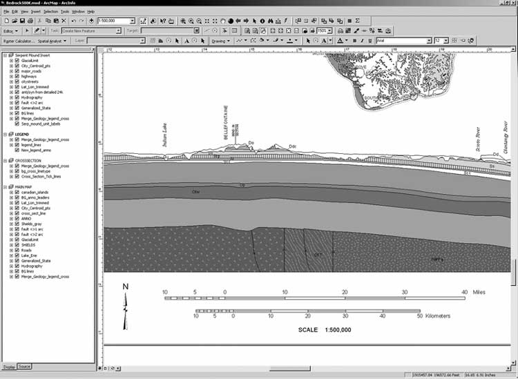Figure 6. The cross section from the new state bedrock geology map is a GIS data layer.

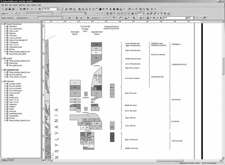Figure 7. The correlation chart from the new state bedrock geology map is a GIS data layer.

A 1:500,000-scale bedrock topography GIS data layer and plot-on-demand map also were compiled digitally by the ODGS. Compilation of the statewide bedrock topography layer presented unique problems because of the different vintages of the original maps and the variety of contour intervals (5, 10, 20, 25, 50, and 100 feet) that had to be used across the state depending on the gradient of relief on the bedrock surface. These difficulties prevented the statewide usage of this data set; it was necessary to recompile the bedrock topography. The 1:24,000-scale bedrock topography contours from the GIS data set were used as the source for the newly compiled data layer. The contours were regridded, at a spacing of 60 meters, to produce a consistent bedrock topography GIS layer. To produce a bedrock topography surface across the entire state, the shaded surface-elevation grid of the state (Powers, Laine, and Pavey, 2002) was clipped to the edge of the bedrock topography grid. The clipped surface-elevation grid, which shows the unglaciated portion of the state in southern and southeastern Ohio, was then merged with the bedrock topography grid to produce the bedrock topography surface across the entire state (figure 8, Ohio Division of Geological Survey, 2003).

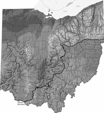Figure 8. The new state bedrock topography map, published at 1:500,000 scale (Ohio Division of Geological Survey, 2003).

SOFTWARE APPLICATION

As the completion of the bedrock geology and bedrock topography GIS conversion projects neared, it became apparent that a methodology had to be developed for data management and data distribution of these large statewide GIS data sets. As part of a contract with ODOT for the completion of the GIS conversion, a multi-use application was created to help manage, distribute, and edit the data and maps. The application was designed with a number of different goals in mind. The application had to be able to extract and set up individual quadrangles for plotting and to extract digital data for public distribution for all 1,576 bedrock geology and bedrock topography maps. The application also had to enable dynamic updating and editing of the data so that versions released to the public are always current.

The application will assist the ODGS in managing and distributing maps and data to the public. One of the application’s functions enables the user to select an individual 7.5-minute quadrangle either by drop-down list of quadrangle names or by selecting it from an index map of quadrangles covering the state of Ohio. Once selected, the bedrock geology or bedrock topography is displayed only for that selected quadrangle (figure 9). Also included are the bedrock topography contours, the bedrock topography data points, and the structure contour maps as TIFF images.

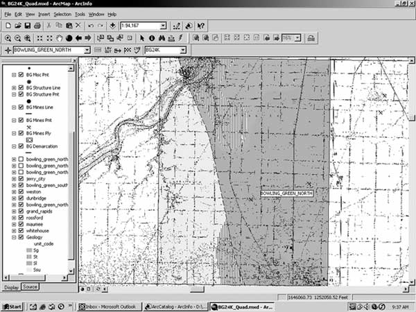Figure 9. Extracted bedrock geology map of the Bowling Green North 7.5-minute quadrangle.

A second function allows for the export of the bedrock geology or bedrock topography data, along with the USGS Digital Raster Graphic base map. The bedrock geology or bedrock topography files are exported in shapefile format, and are written to a temporary directory. Once exported, the data can be distributed to the public.

A third function sets up the map layout for the traditional printing of bedrock geology and bedrock topography maps (figure 10). The layout function takes the extracted bedrock geology data layer, and exports it to a temporary shapefile. The temporary shapefile is then brought back into the map layout for standard symbolization and display. During the setup, the title, authors, and revision date are extracted from a quadrangle metadata database and placed onto the map layout. An inset map is automatically generated during the customized layout process, showing the location of the individual 7.5-minute quadrangle and the state outline. The legend is automatically generated, so that the geologic units will always have the same colors and patterns across the entire state. The legend for the geologic units uses a custom ESRI-style library that was developed for the application. During the quadrangle extraction process, the geologic unit in the attribute table is matched to the custom style in the ESRI-style library.

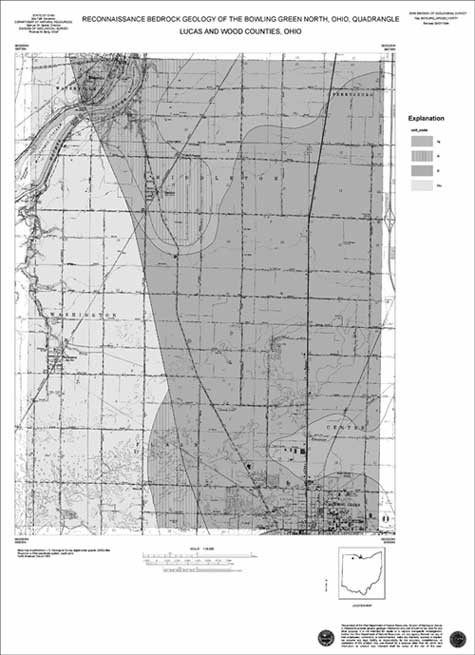Figure 10. Bedrock geology map of the Bowling Green North 7.5-minute quadrangle, set up for plotting at 1:24,000 scale. The title and revision date on the map are extracted from a quadrangle-metadata database.

The fourth function is used only for plotting 1:100,000-scale bedrock geology and bedrock topography maps. This function has the ability to plot 30 × 60-minute blocks of map data that either correspond to a single USGS 1:100,000-scale topographic map, or to an area containing pieces of several USGS topographic maps.

The quadrangle-metadata database is used for multiple purposes. The title, authors, and revision date for the map layout come from the database. The database is used for bibliographic purposes and is used to update the National Geologic Map Database (NGMDB) Map Catalog. Future functions of the application may include placing a standard bibliographic citation on the maps, as obtained from the quadrangle metadata database. Another function may create individual metadata records, so when the map data is exported, customized metadata records can be exported with it.

SUMMARY

ODGS has created the 1:24,000-scale and 1:500,000-scale bedrock geology and bedrock topography GIS data sets, based upon a new set of 1:24,000-scale bedrock geology and bedrock topography maps produced by the ODGS. The resultant 1:500,000-scale bedrock geology map represents the first major revision of the official bedrock geology map of Ohio since 1920. An application has been created for plot-on-demand and data distribution of the bedrock geology and bedrock topography maps. A total of 1,576 individual 7.5-minute quadrangle maps can be extracted from the 1:24,000-scale bedrock geology and bedrock topography data layers. The maps can be set up for printing and the data can also be exported in a compressed (“zipped”) shapefile format and distributed to the public. ODGS plans to extend the application for the extraction and plotting of 1,840 structure contour maps, 220 abandoned underground mine maps, and 120 karst geology maps that have been previously created or that are in preparation.

A quadrangle metadata database has been created to extract the titles, authors, and revision dates for the plotted maps, and to populate the NGMDB. Future implementations could include creating unique metadata records for all the extracted digital data and also creating unique bibliographic citations for all the plotted maps.

The new 1:500,000-scale bedrock geology map will be published in 2004. The new 1:500,000-scale bedrock topography map and the GIS files for the 1:24,000 and 1:500,000-scale bedrock topography recently have been released (Ohio Division of Geological Survey, 2003). Once the printed statewide bedrock geology map is published, the 1:24,000-scale plot-on-demand maps and GIS files for the 1:24,000-scale and 1:500,000-scale bedrock geology also will be released to the public.

REFERENCES

Bernhagen, R.J., 1994, A state geologist’s memories of the Morrow County Boom, in Schafer, W.E., ed., Morrow County, Ohio “Oil Boom” 1961–1967 and the Cambro-Ordovician reservoir of central Ohio: Ohio Geological Society, p. 79–81.

Bownocker, J.A., 1920, Geologic map of Ohio: Ohio Division of Geological Survey Map 1, 1:500,000 scale, 1 sheet.

DeLong, R.M., 1965, Geology of the Kensington quadrangle, Ohio: Ohio Division of Geological Survey Report of Investigations 55, 1 sheet.

Ford, J.P., 1987, Glacial and surficial geology of Cuyahoga County, Ohio: Ohio Division of Geological Survey Report of Investigations 134, 29 p.

Larsen, G.E., 1991, Historical development and problems within the Pennsylvanian nomenclature of Ohio: Ohio Journal of Science, v. 91, p. 69–76.

McDonald, James, 2002, Computer-aided structure-contour mapping in support of the Ohio Division of Geological Survey bedrock-geology program, in Soller, D.R., Digital Mapping Techniques ’02 — Workshop Proceedings: U.S. Geological Survey Open-File Report 02-370, p. 119–127, http://pubs.usgs.gov/of/2002/of02-370/mcdonald.html.

Ohio Division of Geological Survey, 2003, Bedrock-topography data for Ohio: Ohio Division of Geological Survey BG-3, 1 CD-ROM, GIS file format.

Powers, D.M., Laine, J.F., Pavey, R.R., 2002, Shaded elevation map of Ohio: Ohio Division of Geological Survey Map MG-1, 1:500,000 scale.

Sherman, C.E., 1933, Miscellaneous data: Ohio Cooperative Topographic Survey, Volume IV of the Final Report, 327 p.

Swinford, E.M., 1997, Remapping of the bedrock geology of Ohio completed: Ohio Division of Geological Survey, Ohio Geology, Summer 1997, p. 1, 3, http://www.dnr.state.oh.us/geosurvey/oh_geol/97_Summer/remap.htm.

Wickstrom, L.H., McDonald, James, and Berg, T.M., 1998, Working with the Department of Rehabilitation and Correction for the public good: Ohio Division of Geological Survey, Ohio Geology, Summer 1998, p. 1, 3, http://www.dnr.state.oh.us/geosurvey/oh_geol/98_summer/leadart1.htm.