Digital Mapping Techniques '03 — Workshop Proceedings
U.S. Geological Survey Open-File Report 03–471

Delaware Inland Bays Shoreline Extraction Using Landsat 7 Satellite Imagery

By Lillian T. Wang

Delaware Geological Survey, University of Delaware, Delaware Geological Survey Building, Newark, DE 19716
Telephone (302) 831-1096; fax (302) 831-3579; e-mail lillian@udel.edu

INTRODUCTION

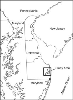
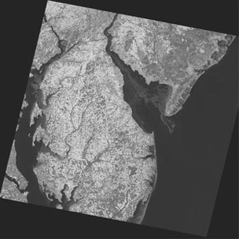
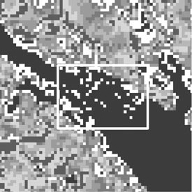
As part of a larger study to map ground-water discharge areas in surface water, Landsat 7 Enhanced Thematic Mapper satellite imagery was used to delineate the coastline for Rehoboth and Indian River Bays, Delaware (fig. 1). Definition of a shoreline was critical in order to isolate pixels that included only open water in the bays. Automated, unbiased methods to extract the shoreline from January 29, 2000 (fig. 2), and February 19, 2002, Landsat images were evaluated. Existing vector shorelines from, for example, the United States Geological Survey (USGS) Digital Line Graphs (DLGs) or the Delaware Land-Use/Land Cover (LULC) data were not used because both vector shorelines are based on data sets that precede the Landsat image acquisition date, both vector shorelines have different resolutions than the Landsat image, and georeferencing errors needed to be minimized during the analysis.

Figure 1. Location of Inland Bays, Delaware.		Figure 2. Landsat image, Path 014 Row 33, January 29, 2000.

Several unsupervised classifications were performed in the Environment for Visualizing Images (ENVI) 3.6 image processing software, using individual bands and band combinations to determine the best spectral wavelength or combination of wavelengths for coastline delineation. The classification of the January Landsat image was initially troubling because known open water in the bays was not classified correctly. It was determined that these misclassified areas were caused by the presence of ice on the bays (fig. 3).

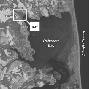Figure 3. Ice located in the northwestern corner of Rehoboth Bay.

IMAGE PROCESSING STEPS

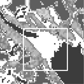
The near-infrared (NIR) and mid-infrared (MIR) wavelength bands normally provide high contrast between land and water (Jensen, 2000). An unsupervised classification of the NIR band classified most of the Inland Bays as water, but there were problem areas such as in the northwestern corner of Rehoboth Bay, shown in figure 4a. MIR wavelength bands were more successful in differentiating land and water because they are sensitive to moisture content (Gibbons and others, 1989; Schneider and Mauser, 1996; Jensen, 2000). However, obviously misclassified pixels still remained in the open water areas (fig. 4b).

Figure 4a. Unsupervised classification of the NIR band (dark pixels = water).		Figure 4b. Unsupervised classification of the MIR bands.

Analysis of all bands seemed to be the next logical step. Visible, NIR and MIR bands were stacked and analyzed using tasseled-cap transformation, a useful tool for compressing spectral data into a few components associated with physical scene characteristics (Crist and Cicone, 1984). The tasseled cap consists of three primary factors: “Brightness” (soil brightness index), “Greenness” (green vegetation index) and “Wetness” (related to soil moisture content). Although used mainly for vegetation studies, tasseled-cap transformation can separate urban, water, and wetland classes (Jensen, 1996).

This transformation resulted in some areas of open water still classified as land, and vice-versa, in the January 29, 2000 image. However, the same process run on the February 19, 2002, image, resulted in very good delineation between land and water. Meteorological data indicated air temperatures at or below freezing several days before the January image was taken. It has been determined that these misclassified areas were ice, and further processing was required to delineate the shoreline.

Classified images often exhibit a lack of spatial coherency. A post-classification technique called sieve classes is used to solve the problem of isolated pixels occurring in classified images, leaving unclassified black pixels. The clump classes technique is then used to clump adjacent similar classified areas, where unclassified pixels are reclassified (fig. 5). Results were converted to an ENVI polygon vector layer, and the water class was exported to an ESRI shapefile. Minor problem areas still existed, and the results were manually edited in ArcGIS using a false-color composite as a base map for visual aid.

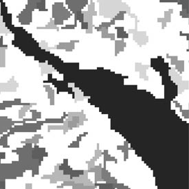Figure 5. Result after sieve and clump classes run on figure 4b.

SUMMARY

Shorelines from older DLG and LULC datasets were not used to delineate a coastline for Rehoboth and Indian River Bays because they were derived from data several years older and have a different spatial resolution than the satellite image. The final, post-processed shoreline is specific to the January 29, 2000, Landsat 7 image, and excludes land pixels as seen in the DLG (figure 6) and LULC shoreline datasets. The tasseled-cap transform was sufficient for shoreline extraction, but the mid-infrared band combination provided the best delineation of the coastline when ice was present on the surface water. Problems encountered in this study were found to be image-specific, due to cold weather conditions in January forming ice on the Inland Bays, Delaware.

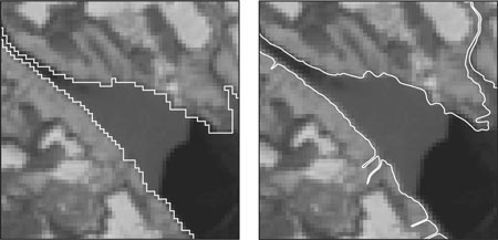Figure 6. Final shoreline (left) compared to USGS DLG 1993 shoreline (right).

ACKNOWLEDGEMENT

This research is funded by the US EPA ą Science to Achieve Results (STAR) Program under grant R826945.

REFERENCES

Crist, E.P., and Cicone, R.C., 1984, A physically-based transformation of Thematic Mapper data — the TM Tasseled Cap: IEEE Transactions on Geosciences and Remote Sensing, GE-22, p. 256–263.

Gibbons, D.E., Wekelic, G.E., Leighton, J.P. and Doyle, M.J., 1989, Application of Landsat Thematic Mapper data for coastal thermal plume analysis at Diablo Canyon: Photogrammetric Engineering and Remote Sensing, v. 55, p. 903–909.

Jensen, J.R., 1996, Introductory digital image processing, (2nd ed.ed.): Upper Saddle River, NJ, Prentice Hall p. 184.

Jensen, J.R., 2000, Remote sensing of the environment — An earth resource perspective: Upper Saddle River, NJ, Prentice Hall, pp. 194, 382.

Schneider, K., and Mauser, W., 1996, Processing and accuracy of Landsat Thematic Mapper data for lake surface temperature measurement: International Journal of Remote Sensing, v. 17, p. 2027–2041.

The Environment for Visualizing Images (ENVI) — Research Systems, Inc., 4990 Pearl East Circle, Boulder, CO 80301 USA, (303) 786-9900, http://www.rsinc.com/.

ESRI, ArcGIS — Environmental Systems Research Institute, Inc., 380 New York St., Redlands, CA 92373-8100 USA, (909) 793-2853, http://www.esri.com/.