
Multifractal IDW Interpolation
Universal Kriging Interpolation
The chemical data for stream sediments and waters has been interpolated in grid format to provide a graphical visualization of the regional variation in chemical values. Spatial interpolation is commonly addressed using methods such as kriging, inverse distance weighting, and fitting polynomial, spline, and Fourier series functions to the data to be interpolated. Inverse distance weighting (IDW) and kriging techniques have been recommended in studies comparing interpolation methods (Weber and Englund, 1992, 1994; Englund, Weber, and Leviant, 1992) and both methods are used in this report to compare the results of the different interpolation methods. IDW is a technique that fits the source data accurately and preserves local anomalies in the interpolation grid. Kriging techniques assume the source data have regionalized errors of estimation and generalize the data to minimize estimation variance. Kriging tends to eliminate local anomalies from the interpolation grid to portray a more general trend for the data.
4.1.0 Grid Map Cell Size, Projection, and legend parameters
Grid cells for both interpolation methods were determined by the default settings of the respective geostatistical packages used to calculate the grid cell values, and differed by a size of 0.5 km2. Grid cell size for each interpolation grid, produced by the GeoDAS System multifractal IDW interpolation (Cheng 2003), is approximately 1 km2. Grid cell size for the kriging interpolations grids used the default size for the ArcGIS 8 Geostatistical Analyst extension universal kriging interpolation, which is approximately 1.5 km2.
Arcview 3.2 was used to display the final maps, using the Albers Equal-Area Conic map projection with the following parameters: Clarke 1866 geoid, Central Meridian: -71, Reference Latitude: 23, Standard Parallel 1: 29.5, Standard Parallel 2: 45.5, False Easting: 0, False Northing: 0.
The legends for the interpolation grid maps are based on percentiles of the original point data, with the cutoffs between the color-categories being the 20th, 30th, 40th, 50th, 60th, 70th, 80th, 90th, and 95th percentile values.
The geochemical units portrayed in the interpolation grid maps are described below:
Stream Sediments:
• Major elements (8)); values expressed as oxide weight percent.
• Trace elements (16); values in mg element/kg sample, which is equivalent to parts-per-million (ppm).
• Trace-element ratios (1);. Unitless ratio.
Stream Waters:
• pH, values expressed as –log10 of hydrogen ion activity.
• Alkalinity and Specific Conductance; units defined in Section 3.2.
4.1.1 Multifractal IDW interpolation
Multifractal inverse distance weighting (IDW) data interpolation was used to generate one set of interpolation grid maps, using the GeoDAS System (phase III) software (Cheng, 2003). IDW interpolation assigns weights to neighboring known values based on distance to the prediction grid cell. The neighbors used in the interpolation of a specific cell value were determined by the default window size setting for the procedure in GeoDAS.
The general IDW spatial model is as follows:

where ![]() is the interpolated chemical value, s0 is
the prediction grid cell (x,
y coordinates), Z is the
known chemical value at the spatial location sj, and lj is the weight given to the known measurement
based on distance from sj to s0 (Johnston, et. al 2001).
is the interpolated chemical value, s0 is
the prediction grid cell (x,
y coordinates), Z is the
known chemical value at the spatial location sj, and lj is the weight given to the known measurement
based on distance from sj to s0 (Johnston, et. al 2001).
Multifractal IDW interpolation estimates the distribution of chemical values based on fitted power law trends between chemical value and grid area using the observed data points. For a detailed discussion on multifractal IDW data interpolation, see Cheng (2003, Appendix C) and Agterberg (2001). Unlike kriging and some other methods, multifractal IDW preserves the local variability of the observed points by assigning greater weights to known outlier values (as opposed to smoothing them). Multifractal IDW is a useful data interpolation method for representing geochemical data, which is highly variable and often contains anomalies (Cheng, 2003).
The multifractal IDW interpolation maps for stream sediment and water chemistry are provided in Section 6.0.
4.1.1.1 Uncertainty in spatial interpolation of geochemical data by multifractal IDW method
The performance of inverse distance weighted multifractal interpolation is tested for the sparsely sampled regional geochemistry dataset by randomly removing samples from the dataset, interpolating the data at the remaining sample sites, and comparing the measured concentration at the removed sites with their respective interpolated values. Each dataset was performance tested five times by randomly removing 15% of the sample sites. For each of the datasets for each variable, more than half of the sample sites were removed and tested at least once in the performance evaluation. The test datasets are interpolated using the same methodology as the final interpolation grid maps, generating a set of plausible grid models of regional geochemistry that are used to calculate standard deviation estimates (interpolation uncertainty) for the entire dataset and by spatial location. The overall interpolation uncertainty for each variable is listed in Table 3 (Section 4.2.3) and the performance test results are portrayed as grids of interpolation uncertainty over the region. The interpolation uncertainty maps for multifractal IDW interpolation are provided in Section 6.0.
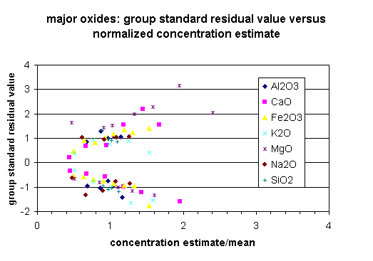
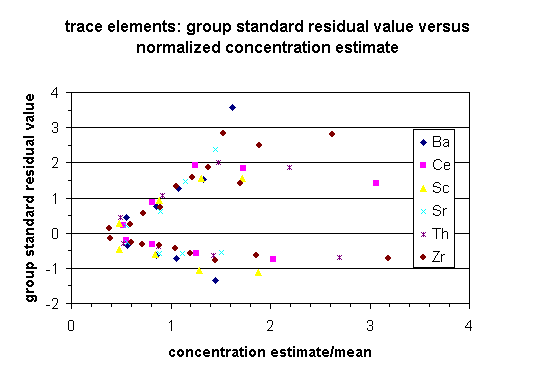
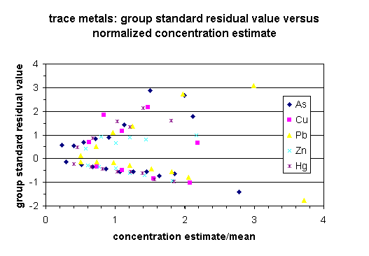
The overall performance (interpolation uncertainty) of the interpolation grids, expressed as the square root of the prediction variance, is positively correlated with the standard deviation of the measured variable in the sample dataset (Table 3 in Section 4.2.3). To test whether the variation of the residuals within individual data sets vary as a function of concentration (heteroscedastic variance), standardardized residual values for the performance test data were calculated for observations grouped by equal concentration intervals for individual data sets. The standardized residual value is calculated as the observed minus predicted group value divided by the square root of the residual mean square for the data set. Separate standardized residual values were calculated for positive and negative deviation from the estimated value for each concentration interval group. The results of this variance test are shown in plots of the standardardized residual value of the concentration interval versus the standardized estimated concentration for the group (Figures 1-3). Figures 1-3 group the data sets into major element, trace element, and trace metal categories; this allows data trends to be easily seen. All data shows similar ranges of standardized residual value and standardized estimated concentration. All data, with the exception of Al2O3, SiO2, and Na2O appear to be heteroscedastic where he absolute value of the standardized residual value increases with increasing concentration.


![]()

![]() 4.1.2
Universal Kriging interpolation
4.1.2
Universal Kriging interpolation
Universal kriging is used as an alternative interpolation method. This technique provides a more general representation of regional patterns in geochemistry as compared to IDW interpolation. Universal kriging is used for spatial prediction in settings where the data are expected follow a trend, varying in both mean (expected value) and variance by location (Johnston, et. al. 2001). The use of universal kriging in this geochemical study is supported by the geochemical variation in the stream sediment and water chemistry data categorized by bedrock lithology group across the study area (box plots by bedrock lithology in Section 6.0). The universal kriging technique applies a trend surface (i.e. a moving average value) to the study area using five local neighbors in the prediction of values at a spatial location (five is the default setting offered by ArcGIS 8 Geostatistical Analyst extension). In this respect, universal kriging is a more powerful technique than other kriging methods (such as ordinary kriging), as it accounts for data variation by this nonrandom trend surface (Johnston, et. al. 2001).
Universal kriging uses the spatial model:

where again ![]() is
the interpolated chemical value of the grid cell, s0 is the
spatial location of the prediction grid cell (x, y coordinates), Fb
is the trend function, and e is a random error value assigned to
the particular grid cell (Pebesma, 1998). The error values are used to fit a
distance vs. direction model between measured points in a semivariogram.
The trend function is added to this error model to produce the final grid interpolation
(Johnston, et. al. 2001). The universal kriging interpolation maps are
provided in Section 6.0.
is
the interpolated chemical value of the grid cell, s0 is the
spatial location of the prediction grid cell (x, y coordinates), Fb
is the trend function, and e is a random error value assigned to
the particular grid cell (Pebesma, 1998). The error values are used to fit a
distance vs. direction model between measured points in a semivariogram.
The trend function is added to this error model to produce the final grid interpolation
(Johnston, et. al. 2001). The universal kriging interpolation maps are
provided in Section 6.0.
Kriging interpolation assumes the dataset has a stationary condition. Universal kriging allows for a weak stationary condition, where the mean and variance may vary regularly with location (Henley, 2001). The log values for stream sediment and water chemistry data were used in the interpolation to normalize the data in order to meet this condition, and converted back to the original values in the map legends. The legends for the universal kriging interpolation grid maps use the same value breaks as the multifractal IDW interpolation maps (20th, 30th, 40th, 50th, 60th, 70th, 80th, 90th, and 95th percentile values), This allows for an easy comparison of results between the two grid interpolation methods.
4.1.2.1 Uncertainty in spatial interpolation of geochemical data by kriging method
The performance of the universal kriging interpolation method is calculated using the estimation variance generated during the model fit of the semivariogram, producing a standard error map. These grids were generated using the universal kriging standard error map function within the ArcGIS Geospatial Analyst extension. The logarithmic transform was used to calculate the standard error maps for the heteroscedastic data sets, as the absolute magnitude of the residual values increases with increasing estimated concentration (Figures 1-3). The interpolation uncertainty maps for universal kriging interpolation are provided in Section 6.0. The trend function formulated in universal kriging may be overestimated, which can lead to a degree of inaccuracy in uncertainty (Johnston, et. al. 2001), however the goal of this technique to provide a general regional pattern is maintained. The legends for the universal kriging interpolation grid maps use the same value breaks as the multifractal IDW interpolation maps, in order to easily compare the results.
4.2 Geochemical Statistics
4.2.1 Box Plots
Box plots of the chemical data, grouped by bedrock lithology group categories, show the 5th, 25th, 50th, 75th, and 95th percentiles for the chemical data for each lithology group.
4.2.2 Geochemical Statistics, by bedrock lithology groups, drainage basin, and population density
Median values are generally the best measure of central tendency in regional geochemical datasets (Reimann and Filzmoser, 2000). Median values of the chemical data were calculated for map polygon areas using the Point-Stat-Calc extension for ArcView v.3.2 (Dombroski, 2000). Stream sediment and water sample sites are grouped by polygons representing individual rock lithology groups and hydrologic basins in New England. Stream sediment data for base metals (Cu, Hg, Pb, Zn), which are commonly found in areas of human infrastructure, are also grouped by population density categories.
The legends for the median-value maps are based on the standard deviation of the range in median values of data for each of the polygons of grouped stream sediment sample sites. The cutoffs between the color-categories for each map are the standard deviation intervals (–3, -2, -1, 0, 1, 2, 3) about the average of median values.
4.2.3 Descriptive Statistics and QQ plots
Descriptive statistics of the stream sediment and water chemistry data are provided in Table 3. Quantile-Quantile (QQ) plots of the stream sediment and water chemistry data are provided to display the distribution patterns of the data. QQ plots compare ordered values of a variable with quantiles of a theoretical distribution. Normal and lognormal theoretical distributions are used in the QQ plots in this report. If the data are normally (or lognormally) distributed with mean (u) and standard deviation (s), the data points on the QQ plot should lie approximately on a straight line with intercept u and slope s. Curvature of the trend of points indicates departures from normality. The standard normal scores are calculated by taking the Z-score of the data ranked by ascending order. The Z-scores are the inverse values of the standard normal cumulative distribution, based on the probability p= rank value-0.5/rank value* total N samples.
|
Units |
Mean |
Std. Dev. |
Minimum |
Maximum |
Geom. Mean |
Median |
IQR |
Interpolation Uncertanity |
|
|---|---|---|---|---|---|---|---|---|---|
|
Major Elements (expressed as oxides) |
|||||||||
|
Al2O3 |
wt. % |
9.94 |
1.81 |
3.21 |
21.08 |
9.76 |
10.02 |
2.00 |
1.48 |
|
CaO |
wt. % |
1.87 |
1.05 |
0.13 |
11.56 |
1.64 |
1.64 |
1.08 |
0.78 |
|
Fe2O3 |
wt. % |
3.55 |
1.60 |
0.35 |
14.56 |
3.21 |
3.31 |
2.05 |
1.21 |
|
K2O |
wt. % |
1.74 |
0.60 |
0.40 |
5.23 |
1.64 |
1.69 |
0.72 |
0.38 |
|
MgO |
wt. % |
0.93 |
0.54 |
0.05 |
4.75 |
0.78 |
0.82 |
0.67 |
0.40 |
|
Na2O |
wt. % |
2.02 |
0.50 |
0.22 |
3.98 |
1.96 |
2.02 |
0.63 |
0.35 |
|
SiO2 |
wt. % |
70.18 |
5.92 |
45.08 |
91.82 |
69.92 |
70.42 |
7.31 |
5.21 |
|
TiO2 |
wt. % |
1.10 |
0.58 |
0.21 |
7.15 |
0.99 |
0.94 |
0.58 |
0.44 |
Trace Elements |
|||||||||
|
As |
ppm |
5.08 |
7.06 |
0.30 |
98.30 |
2.85 |
2.80 |
4.70 |
6.95 |
|
Ba |
ppm |
330.57 |
106.67 |
101.70 |
1178.99 |
314.75 |
315.49 |
117.88 |
83.65 |
|
Ce |
ppm |
106.74 |
77.49 |
20.00 |
842.00 |
90.15 |
83.00 |
62.25 |
61.45 |
|
Cu |
ppm |
12.13 |
8.59 |
1.00 |
151.00 |
10.25 |
10.00 |
8.00 |
8.01 |
|
Hg |
ppm |
0.06 |
0.11 |
0.00 |
2.75 |
0.04 |
0.04 |
0.03 |
0.05 |
|
La |
ppm |
53.72 |
41.38 |
9.00 |
457.00 |
44.47 |
41.00 |
34.00 |
32.41 |
|
Nd |
ppm |
47.38 |
36.89 |
4.50 |
410.00 |
39.05 |
37.00 |
29.00 |
29.87 |
|
Pb |
ppm |
44.14 |
69.96 |
2.00 |
1170.00 |
33.41 |
30.00 |
17.00 |
49.24 |
|
Sc |
ppm |
9.78 |
4.50 |
1.00 |
30.00 |
8.81 |
9.00 |
5.00 |
3.14 |
|
Sr |
ppm |
156.92 |
72.53 |
39.48 |
844.71 |
143.93 |
146.30 |
70.83 |
53.68 |
|
Th |
ppm |
18.80 |
17.03 |
3.00 |
186.00 |
13.92 |
13.00 |
14.00 |
12.98 |
|
U |
ppm |
4.83 |
4.57 |
0.10 |
59.60 |
3.75 |
3.60 |
3.30 |
4.50 |
|
V |
ppm |
55.53 |
25.37 |
5.00 |
197.00 |
49.63 |
53.00 |
35.00 |
18.40 |
|
Y |
ppm |
36.53 |
22.48 |
5.21 |
385.01 |
32.49 |
30.93 |
18.60 |
17.46 |
|
Zn |
ppm |
49.82 |
37.42 |
3.00 |
692.00 |
42.29 |
43.00 |
28.00 |
31.47 |
|
Zr |
ppm |
722.57 |
660.57 |
77.61 |
11572.35 |
574.13 |
535.12 |
450.96 |
448.80 |
Surface Water Chemistry |
|||||||||
|
Alkalinity |
* |
0.47 |
0.71 |
0.00 |
7.30 |
0.20 |
0.42 |
0.35 |
|
|
Specific Conductance |
* |
148.57 |
1211.78 |
1.00 |
42000.00 |
62.52 |
57.00 |
79.00 |
0.30 |
|
pH |
* |
6.76 |
0.87 |
3.10 |
10.40 |
6.70 |
6.70 |
1.10 |
0.64 |
(* for unit measurement details see Surface Water Chemistry (3.2) in Section 3.0)
Direct questions and comments to:
Gilpin R. Robinson
U.S. Geological Survey
Email grobinso@usgs.gov
Phone (703)-648-6113