Sediment-Texture Units of the Sea Floor for Buzzards Bay, Massachusetts (BuzzardsBay_sedcover, polygon shapefile, Geographic, WGS84)

Metadata also available as - [Outline] - [XML] - [DIF]

Frequently anticipated questions:


What does this data set describe?

Title:
Sediment-Texture Units of the Sea Floor for Buzzards Bay, Massachusetts (BuzzardsBay_sedcover, polygon shapefile, Geographic, WGS84)
Abstract:
Geologic, sediment texture, and physiographic zone maps characterize the sea floor of Buzzards Bay, Massachusetts. These maps were derived from interpretations of seismic-reflection profiles, high-resolution bathymetry, acoustic-backscatter intensity, bottom photographs, and surficial sediment samples. The interpretation of the seismic stratigraphy and mapping of glacial and Holocene marine units provided a foundation on which the surficial maps were created. This mapping is a result of a collaborative effort between the U.S. Geological Survey and the Massachusetts Office of Coastal Zone Management to characterize the surface and subsurface geologic framework offshore of Massachusetts.
  1. How might this data set be cited?
    Foster, David S., 2014, Sediment-Texture Units of the Sea Floor for Buzzards Bay, Massachusetts (BuzzardsBay_sedcover, polygon shapefile, Geographic, WGS84): Open-File Report 2014-1220, U.S. Geological Survey, Coastal and Marine Geology Program, Woods Hole Coastal and Marine Science Center, Woods Hole, MA.

    Online Links:

    This is part of the following larger work.

    Foster, David S., Baldwin, Wayne E., Barnhardt, Walter A., Schwab, William C., Ackerman, Seth D., Andrews, Brian D., and Pendleton, Elizabeth A., 2014, Shallow Geology, Sea-Floor Texture, Physiographic Zones of Buzzards Bay, Massachusetts: Open-File Report 2014-1220, U.S. Geological Survey, Reston, VA.

    Online Links:

  2. What geographic area does the data set cover?
    West_Bounding_Coordinate: -71.122548
    East_Bounding_Coordinate: -70.612718
    North_Bounding_Coordinate: 41.766648
    South_Bounding_Coordinate: 41.369362
  3. What does it look like?
    https://pubs.usgs.gov/of/2014/1220/GIS_catalog/SedimentTexture/BuzzardsBay_sedcover_browse.png (PNG)
    Image of the sediment texture and distribution shapefile for Buzzards Bay
  4. Does the data set describe conditions during a particular time period?
    Beginning_Date: 01-Jan-2004
    Ending_Date: 31-Aug-2011
    Currentness_Reference:
    ground condition of the source data that this interpretation is based on
  5. What is the general form of this data set?
    Geospatial_Data_Presentation_Form: vector digital data
  6. How does the data set represent geographic features?
    1. How are geographic features stored in the data set?
      This is a Vector data set. It contains the following vector data types (SDTS terminology):
      • G-polygon (1149)
    2. What coordinate system is used to represent geographic features?
      Horizontal positions are specified in geographic coordinates, that is, latitude and longitude. Latitudes are given to the nearest 0.000001. Longitudes are given to the nearest 0.000001. Latitude and longitude values are specified in Decimal degrees. The horizontal datum used is D_WGS_1984.
      The ellipsoid used is WGS_1984.
      The semi-major axis of the ellipsoid used is 6378137.000000.
      The flattening of the ellipsoid used is 1/298.257224.
  7. How does the data set describe geographic features?
    BuzzardsBay_sedcover
    Sediment Cover shapefile for Buzzards Bay (Source: U.S. Geological Survey)
    FID
    Internal feature number. (Source: ESRI) Sequential unique whole numbers that are automatically generated.
    Shape
    Feature geometry. (Source: Esri) Coordinates defining the features.
    data_confi
    Each interpreted polygon was assigned a data interpretation confidence value from 1-4 on the basis of the quality and number of input data sources. (Source: U.S. Geological Survey)
    ValueDefinition
    1Sediment texture regions that were defined on the basis of the highest resolution bathymetry (10m) and backscatter (1m), bottom photos, sediment samples with laboratory analysis, and seismic interpretations were given the highest data interpretation confidence value of 1.
    2Sediment texture regions that were defined on the basis of the highest resolution bathymetry (10m) and backscatter (1m), bottom photos, qualitative descriptions of sediment samples, and seismic interpretations were given the data interpretation confidence value of 2
    3Sediment texture regions that were defined on the basis of low resolution single beam bathymetry and sediment samples descriptions were given the data interpretation confidence value of 3. Exceptions occur for three polygons (FID 917, 932 and 1148) where only one laboratory sample is in each polygon. These polygons were not included in confidence level 2 where high quality geophysical data exists.
    4Sediment texture regions that were defined on the basis of low resolution single beam bathymetry were given the lowest (4) data interpretation confidence value of 4
    sed_type
    Bottom-type classification on the basis of twelve composite units that represent combinations of four end-member units (R= rock; G= gravel; S= sand; M= mud). (Source: Barnhardt and others (1998))
    ValueDefinition
    RThe end-member texture (= or > 90%) Rock (R) is the primary texture.
    GThe end-member texture (= or > 90%) Gravel (G) is the primary texture.
    GsThe dominant texture (> 50%) Gravel (G) is given the upper case letter and the subordinate texture (< 50%) sand (s) is given a lower case letter.
    SThe end-member texture (= or > 90%) Sand (S) is the primary texture.
    SgThe dominant texture (> 50%) Sand (S) is given the upper case letter and the subordinate texture (< 50%) gravel (g) is given a lower case letter.
    SmThe dominant texture (> 50%) Sand (S) is given the upper case letter and the subordinate texture (< 50%) mud (m) is given a lower case letter.
    MsThe dominant texture (> 50%) Mud (M) is given the upper case letter and the subordinate texture (< 50%) sand (s) is given a lower case letter.
    MThe end-member texture (= or > 90%) Mud (M) is the primary texture.
    RgThe dominant texture (> 50%) Rock (R) is given the upper case letter and the subordinate texture (< 50%) gravel (g) is given a lower case letter.
    RsThe dominant texture (> 50%) Rock (R) is given the upper case letter and the subordinate texture (< 50%) sand (s) is given a lower case letter.
    RmThe dominant texture (> 50%) Rock (R) is given the upper case letter and the subordinate texture (< 50%) mud (m) is given a lower case letter.
    GrThe dominant texture (> 50%) Gravel (G) is given the upper case letter and the subordinate texture (< 50%) rock (r) is given a lower case letter.
    SrThe dominant texture (> 50%) Sand (S) is given the upper case letter and the subordinate texture (< 50%) rock (r) is given a lower case letter.
    MrThe dominant texture (> 50%) Mud (M) is given the upper case letter and the subordinate texture (< 50%) rock (r) is given a lower case letter.
    simple
    sediment nomenclature on the basis of 3 simple classes: sand, mud, hardbottom as defined in the CZM sample database (Source: U.S. Geological Survey)
    ValueDefinition
    sandSediment whose primary component (> 50%) is sand
    hardbottomSediment whose primary component is rock, boulder, cobble, or coarse gravel
    mudSediment whose primary component (> 50%) is silt and clay
    phi_class
    Sediment class as defined by Wentworth classification determined using laboratory analyzed samples in the CZM sample database. Null values are indicated as -999. (Source: Wentworth (1922))
    ValueDefinition
    coarse pebblessediment class whose phi size is between -4 and -5
    coarse siltsediment class whose phi size is between 4 and 5
    coarse sandsediment class whose phi size is between 0 and 1
    cobblesediment class whose phi size is between -6 and -8
    fine pebblessediment class whose phi size is between -2 and -3
    fine sandsediment class whose phi size is between 2 and 3
    fine siltsediment class whose phi size is between 6 and 7
    granulessediment class whose phi size is between -1 and -2
    medium pebblessediment class whose phi size is between -3 and -4
    medium sandsediment class whose phi size is between 2 and 1
    medium siltsediment class whose phi size is between 5 and 6
    very coarse pebblessediment class whose phi size is between -5 and -6
    very coarse sandsediment class whose phi size is between 0 and -1
    very fine sandsediment class whose phi size is between 3 and 4
    very fine siltsediment class whose phi size is between 7 and 8
    N/Asediment class whose phi size could not be determined from grain size data or there were no samples with laboratory analyzed grain size statistics within the polygon
    Area
    Area of feature in kilometers squared using UTM, zone 19, WGS 84. (Source: Esri)
    Range of values
    Minimum:0.000069
    Maximum:132.783
    Units:kilometers
    Resolution:0.000001
    Count_
    The number of sediment samples (with laboratory analyzed grain size statistics) that occur within each qualitatively-derived polygon. This field is automatically generated by Esri when point data (sample database) is joined to a polygon (sediment texture interpretation). A value of zero indicates there are no samples within that polygon. (Source: Esri)
    Range of values
    Minimum:0
    Maximum:56
    Units:count
    Resolution:1
    Avg_Gravel
    Average percent weight (%) gravel (as determined from samples with laboratory analyzed grain size statistics) within each qualitatively derived polygon. This field was automatically generated by Esri as a summary of the numeric attributes of the points that fall inside a polygon when point data (sample database) is joined to a polygon (sediment texture interpretation). (Source: U.S. Geological Survey)
    Range of values
    Minimum:0
    Maximum:74.45
    Units:percent
    Avg_Sand
    Average percent weight (%) sand within each qualitatively derived polygon. This field was automatically generated by Esri as a summary of the numeric attributes of the points that fall inside a polygon when point data (sample database) is joined to a polygon (sediment texture interpretation). (Source: U.S. Geological Survey)
    Range of values
    Minimum:5.94
    Maximum:99.73
    Units:percent
    Avg_Silt
    Average percent weight (%) silt within each qualitatively derived polygon. This field was automatically generated by Esri as a summary of the numeric attributes of the points that fall inside a polygon when point data (sample database) is joined to a polygon (sediment texture interpretation). (Source: U.S. Geological Survey)
    Range of values
    Minimum:0
    Maximum:71.25
    Units:percent
    Avg_Clay
    Average percent weight (%) clay within each qualitatively derived polygon. This field was automatically generated by Esri as a summary of the numeric attributes of the points that fall inside a polygon when point data (sample database) is joined to a polygon (sediment texture interpretation). (Source: U.S. Geological Survey)
    Range of values
    Minimum:0
    Maximum:37.64
    Units:percent
    Avg_PHI
    Average phi size within each qualitatively derived polygon (-999 is a no data value, which means there were no samples with laboratory analyzed grain size statistics within that polygon) (Source: U.S. Geological Survey)
    Range of values
    Minimum:-3.41
    Maximum:7.09
    Units:phi
    Resolution:0.01
    MEAN
    Average water depth (NAVD 88) within each qualitatively derived polygon. (Source: U.S. Geological Survey)
    Range of values
    Minimum:-34.61
    Maximum:-0.931
    Units:meters
    Resolution:0.000001

Who produced the data set?

  1. Who are the originators of the data set? (may include formal authors, digital compilers, and editors)
  2. Who also contributed to the data set?
  3. To whom should users address questions about the data?
    David S. Foster
    U.S. Geological Survey
    Geologist
    U.S. Geological Survey
    Woods Hole, MA
    USA

    508-548-8700 x2271 (voice)
    508-457-2310 (FAX)
    dfoster@usgs.gov

Why was the data set created?

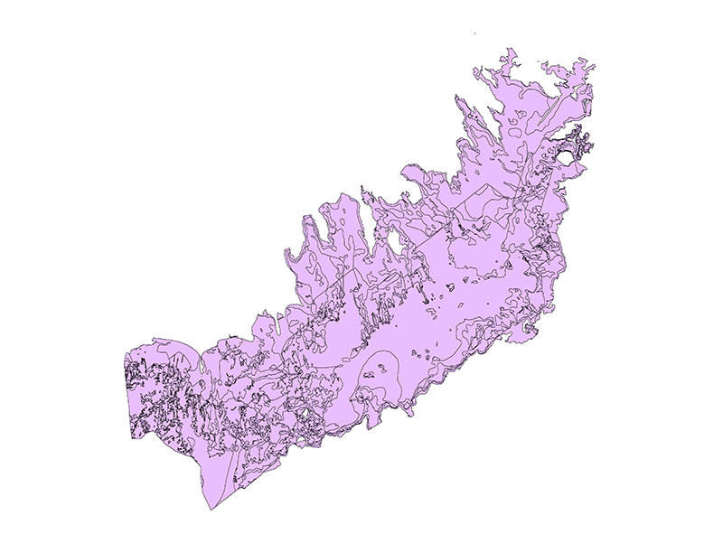
These sea floor sediment cover data were created from geophysical and sample data collected from Buzzards Bay, and are used to characterize the sea floor in the area. Sediment type and distribution maps are important data layers for marine resource managers charged with protecting fish habitat, delineating marine boundaries, and assessing environmental change due to natural or human impacts.

How was the data set created?

  1. From what previous works were the data drawn?
    Poppe and others, 2007 (source 1 of 8)
    Poppe, L.J., Ackerman, S.D., Foster, D.S., Blackwood, D.S., Butman, B., Moser, M.S., and Stewart, H.F., 2007, Sea-floor character and surface processes in the vicinity of Quicks Hole, Elizabeth Islands, Massachusetts: Open-File Report 2006-1357, U.S. Geological Survey, Reston, VA.

    Online Links:

    Type_of_Source_Media: online
    Source_Contribution:
    This publication provides the source geophysical (backscatter and bathymetry) and bottom photographs and sediment samples for the Quicks Hole area of Buzzards Bay. Two 29-foot launches deployed from the NOAA Ship Thomas Jefferson were used to acquire bathymetric and backscatter data during 2004. The multibeam bathymetric data were collected with hull-mounted 455-kHz RESON 8125 and 240-kHz RESON 8101 systems. The sidescan sonar data were acquired with a hull-mounted Klein 5250 system operating at 100 kHz. Sediment samples and bottom photos were collected aboard the R/V Rafael with a modified Van Veen grab sampler and SEABOSS, respectively.
    Pendleton and others, 2012 (source 2 of 8)
    Pendleton, E.A., Twichell, D.C., Foster, D.S., Worley, C.R, Irwin, B.J., and Danforth, W.W., 2012, High-resolution geophysical data from the sea floor surrounding the Western Elizabeth Islands, Massachusetts: Open-File Report 2011-1184, U.S. Geological Survey, Reston, VA.

    Online Links:

    Type_of_Source_Media: online
    Source_Contribution:
    This report provided source geophysical (sidescan, bathymetry, and seismic-reflection profiles) for the area of Buzzards Bay surrounding the western Elizabeth Islands. Surveying was conducted aboard the RV Rafael in September 2010. Interferometric-sonar, sidescan-sonar, and chirp seismic-reflection systems were deployed simultaneously during the cruise. Bathymetric sounding data were collected with an SEA SWATHplus 234-kilohertz (kHz) interferometric sonar system. Sidescan-sonar (acoustic-backscatter) data were acquired with a Klein 3000 dual-frequency (100 and 500 kHz) sidescan-sonar system. High-resolution chirp seismic-reflection profiles were collected using an EdgeTech Geo-Star full spectrum sub-bottom (FSSB) system and SB-424 towfish.
    Turecek and others, 2012 (source 3 of 8)
    Turecek, A.M., Danforth, W.W., Baldwin, W.E., and Barnhardt, W.A., 2012, High-resolution geophysical data collected within Red Brook Harbor, Buzzards Bay, Massachusetts, in 2009: Open-File Report 2010-1091, U.S. Geological Survey, Reston, VA.

    Online Links:

    Type_of_Source_Media: online
    Source_Contribution:
    This report provided the source geophysical (sidescan, bathymetry, and seismic-reflection profiles), sediment sample and bottom photograph data for Buzzards Bay in the area of Red Brook Harbor. Surveying was conducted aboard the R/V Rafael. Bathymetric data were collected with an SEA SWATHplus 234-kilohertz (kHz) interferometric sonar system. Acoustic backscatter, a measure of the intensity of returns from an insonified area of the sea floor, was recorded by the SEA SWATHplus interferometric sonar system. Seismic-reflection profiles were collected with a Knudsen Engineering, Ltd. (KEL) Chirp 3202 dual-frequency (centered at 3.5- and 200-kHz) Chirp system. The USGS Mini SEABed Observation and Sampling System (Mini SEABOSS) was used to collect digital photography and video and sediment samples
    Ackerman and others, 2013 (source 4 of 8)
    Ackerman, S.D., Andrews, B.D., Foster, D.S., Baldwin, W.E., and Schwab, W.C., 2013, High-Resolution Geophysical Data from the Inner Continental Shelf: Buzzards Bay, Massachusetts: Open-File Report 2012-1002, U.S. Geological Survey, Reston, VA.

    Online Links:

    Type_of_Source_Media: online
    Source_Contribution:
    This report provided the source geophysical (sidescan, bathymetry, and seismic-reflection profiles) for Buzzards Bay. The mapping was conducted during research cruises aboard the NOAA Ship RUDE (2004), the Megan T. Miller (2009 and 2010) and the Scarlett Isabella (2011). The NOAA Ship RUDE acquired bathymetric soundings in 2004 using a RESON SeaBat 8125 455-kHz multibeam-echosounder system. All other surveys used the following systems: bathymetric data were acquired in the Buzzards Bay survey area using a Systems Engineering and Assessment, Ltd. (SEA) SWATHplus-M 234-kilohertz (kHz) interferometric sonar system; acoustic backscatter data were collected with a Klein 3000 dual-frequency sidescan-sonar (132 and 445 kHz); chirp seismic-reflection data were collected in the Buzzards Bay survey area using an EdgeTech Geo-Star FSSB subbottom profiling system and an SB-0512i towfish.
    Pendleton and others, 2014 (source 5 of 8)
    Pendleton, E.A., Andrews, B.D., Danforth, W.W., and Foster, D.S., 2013, High-resolution geophysical data collected aboard the U.S. Geological Survey research vessel Rafael to supplement existing datasets from Buzzards Bay and Vineyard Sound, Massachusetts: Open-File Report 2013-1020, U.S. Geological Survey, Reston, VA.

    Online Links:

    Type_of_Source_Media: online
    Source_Contribution:
    This report provided the source geophysical (sidescan, bathymetry, and seismic-reflection profiles) for Buzzards Bay in the area of Naushon Island and seismic reflection profiles in northeast Buzzards Bay. These areas were surveyed with the RV Rafael in 2010 and 2011. In 2010, seismic-reflection data were acquired with a boomer source and GeoEel 8-channel streamer. Interferometric-sonar, sidescan-sonar, and Knudsen seismic-reflection systems were deployed simultaneously during cruise 2011. Bathymetry data were collected with an SEA SWATHplus 234-kilohertz (kHz) interferometric sonar system. Sidescan-sonar (acoustic-backscatter) data were acquired with a Klein 3000 dual-frequency (100 and 500 kHz) sidescan-sonar system. of high-resolution chirp seismic data were collected using a dual frequency (3.5 and 200 kHz) Knudsen Engineering Limited (KEL) Chirp 3202 system.
    CZM sample database (source 6 of 8)
    Ford, K.H., Huntley, E.C., Sampson, D.W., and Voss, S., Unpublished Material, Massachusetts Sediment Database.

    Other_Citation_Details:
    This sample database has been compiled and vetted from existing samples and datasets by the Massachusetts Office of Coastal Zone Management. The data are currently unpublished, but may be acquired by contacting the CZM office: 251 Causeway St Boston, MA 02114 (617) 626-1000 czm@state.ma.us
    Type_of_Source_Media: digital vector
    Source_Contribution:
    Sediment sample databases of Ford and Voss (2010) and McMullen and others (2011) were combined then edited and supplemented with NOAA chart sampling data and bottom photos and descriptions by a group of GIS specialists at the Massachusetts Office of Coastal Zone Management (Emily Huntley, personal communication). These data contained sediment laboratory statistics when available, visual descriptions if sediment analysis was not performed or if the site was a bottom photograph, and classification fields of Barnhardt and others (1998), Shepard (1954), and Wentworth (1922) as well as average sediment statistics and phi size, when laboratory analysis was conducted.
    Poppe and others, 2008 (source 7 of 8)
    Poppe, L.J., McMullen, K.Y., Foster, D.S., Blackwood, D.S., Williams, S.J., Ackerman, S.D., Barnum, S.R., and Brennan, R.T., 2008, Sea-floor character and sedimentary processes in the vicinity of Woods Hole, Massachusetts: Open File Report 2008-1004, U.S. Geological Survey, Reston, VA.

    Online Links:

    Type_of_Source_Media: online
    Source_Contribution:
    This publication provides the source geophysical (backscatter and bathymetry) and bottom photographs and sediment samples for Woods Hole. Two 29-foot launches deployed from the NOAA Ship Whiting were used to acquire bathymetric and backscatter data during 2001. The bathymetric data were collected with a hull-mounted 240-kHz RESON 8101 shallow-water system aboard launch 1005. The sidescan-sonar data were acquired with a hull-mounted Klein T-5000 system operating at 455 kHz aboard launch 1014. Sediment samples and bottom photos were collected aboard the R/V Rafael with a modified Van Veen grab sampler and SEABOSS, respectively, in 2007.
    Ackerman and others, 2014 (source 8 of 8)
    Ackerman, S.D., Pappal, A.L., Huntley, E.C., Blackwood, D.S., and Schwab, W.C., 2014, Geological Sampling Data and Benthic Biota Classification: Buzzards Bay and Vineyard Sound, Massachusetts: Open file Report 2014-1220, U.S. Geological Survey, Reston, VA.

    Online Links:

    Type_of_Source_Media: online
    Source_Contribution:
    This report provided high-resolution digital photographs of the Buzzards Bay sea floor. At each station, the USGS SEABOSS was towed approximately one meter off the bottom at speeds of less than one knot. Because the recorded position is actually the position of the GPS antenna on the survey vessel, not the SEABOSS sampler, the estimated horizontal accuracy of the sample location is ± 30 meters (m). Photographs were obtained using a Konica-Minolta DiMAGE A2 digital still camera, and continuous video was collected from a Kongsberg Simrad OE1365 high-resolution color video camera, usually for 5 to 15 minutes. These data were important in defining rocky zones where sediment samples do not exist.
  2. How were the data generated, processed, and modified?
    Date: 2013 (process 1 of 4)
    The texture and spatial distribution of sea-floor sediment were qualitatively-analyzed in ArcGIS using several input data sources (listed in the source contribution), including acoustic backscatter, bathymetry, seismic-reflection profile interpretations, bottom photographs, and sediment samples. In order to create the interpretation, first the polygon shapefile of the Massachusetts coast (1:25,000) OUTLINE25K_POLY (http://www.mass.gov/anf/research-and-tech/it-serv-and-support/application-serv/office-of-geographic-information-massgis/datalayers/outline.html) was reprojected from Massachusetts State Plane NAD83 to WGS84 UTM Zone 19N using ArcMap (version 9.3): ArcToolbox -- Data Management Tools -- Projections and Transformations -- Feature -- Project. The polygon was edited so that it enclosed Buzzards Bay and surrounding coastal embayments. The edited shapefile was imported to a file geodatabase as a feature dataset. Then physiographic zone polygons were created using 'cut polygon' and 'auto-complete polygon' in an edit session. In general, polygon editing was done at scales between 1:5,000 and 1:20,000, depending on the size of the traced feature and the resolution of the source data. Separate polygons exist where the adjacent physiographic zones are the same but have different confidence levels. The following numbered steps outline the workflow of the data interpretation.
    1. Backscatter intensity data (available at 1 m resolution) was the first input. Changes in backscatter amplitude were digitized to outline possible changes in sea-floor texture on the basis of acoustic return. Areas of high backscatter (light colors) have strong acoustic reflections and suggests boulders, gravels, and generally coarse sea-floor sediments. Low-backscatter areas (dark colors) have weak acoustic reflections and are generally characterized by finer grained material such as muds and fine sands. 2. The polygons were then refined and edited using gradient, rugosity, and hillshaded relief images derived from interferometric and multibeam swath bathymetry and (available at 10 m resolutions). Areas of rough topography and high rugosity are typically associated with rocky areas, while smooth, low-rugosity regions tend to be blanketed by fine-grained sediment. These bathymetric derivatives helped to refine polygon boundaries where changes from primarily rock to primarily gravel may not have been apparent in backscatter data, but could easily be identified in hillshaded relief and slope changes. 3. The third data input (where available) was the stratigraphic interpretation of seismic-reflection profiles, which further constrained the extent and general shape of sea-floor sediment distributions and rocky outcrops, and also provided insight concerning the likely sediment texture of the feature on the basis of pre-Quaternary, glacial or post-glacial origin. Seismic lines and the surficial geologic maps derived from them and used here as input data were collected at typically 100-meter spacing, with tie-lines generally spaced 1-km apart. 4. After all the sea-floor features were traced from the geophysical data, a new field was created in the shapefile called 'sed_type'. Bottom photographs and sediment samples were used to define sediment texture for the polygons using Barnhardt and others (1998) classification. Some polygons had more than one sample, and some polygons lacked sample information. For multiple samples within a polygon, the dominant sediment texture (or average phi size) was used to classify sediment type (often aided by the 'data join' sediment statistics described in a later processing step). In rocky areas, bottom photos were used in the absence of sediment samples to qualitatively define sediment texture. Polygons that lacked sample information were texturally defined through extrapolation from adjacent or proximal polygons of similar acoustic character that did contain sediment samples. 325 samples of the over 10,625 total within the study area were analyzed in the laboratory for grain size. Samples with laboratory grain size analysis were preferred over visual descriptions when defining sediment texture throughout the study area. Bottom photo stations are typically around 2-km apart, and the density of sediment samples varies throughout the study area, with an average of 1.36 samples per square km, while rocky areas have almost no sediment samples. Person who carried out this activity:
    David S. Foster
    U.S. Geological Survey
    Geologist
    U.S. Geological Survey
    Woods Hole, MA
    USA

    508-5488700 x2271 (voice)
    508-457-2310 (FAX)
    dfoster@usgs.gov
    Data sources used in this process:
    • All
    Date: 2013 (process 2 of 4)
    After some additional qualitative polygon editing and reshaping was done in order to create a sediment map that was in the best agreement with all input data: lidar, bathymetry, backscatter, seismic interpretations, bottom photographs, and sediment samples, 3 more fields were added (ArcMap version 9.3.1). The first field, 'simple' is just 3 classes: sand, mud, or hardbottom. Another field 'phi_class' was created and defined using the Wentworth (1922) sediment classification, and finally, a field 'Data_confi' was added as a data interpretation confidence, which describes how confident we are in the interpretation the basis of the number and quality of the input data sources (see the entity and attribute sections for more information on these fields). The remaining fields contain sediment texture statistics or mean water depth information and were created and populated using data joins or zonal statistics functions within ArcMap (version 9.3.1). The fields beginning with "Avg_" and the "Count_" field were automatically generated by computing a data join where the CZM sample database (vector points) was edited to include only the samples with laboratory sediment analysis and joined to the qualitatively-derived polygon file. Each polygon was given an average of the numeric attributes of the points (with laboratory grain size analysis) that fall inside it, and the count field shows how many laboratory analyzed points fall inside it. 325 samples were analyzed in the laboratory. Several fields that were not wanted were deleted after the join. A mean water depth (NAVD 88) field was created using ArcMap (version 9.3): ArcToolbox ? Spatial Analyst Tools ? Zonal -- Zonal Statistics as Table, where the mean water depth for each polygon (input zone data using the zone field sed_type) was derived from the input raster topographic and bathymetric grid (<https://pubs.usgs.gov/of/2014/1220/GIS_catalog/SourceData/bathy/). No data raster values were ignored in determining the output value for each polygon zone. If all raster values were null within a polygon, that zone had a null value (changed to -999) for that zone. The output was saved to a table, which was joined with the sediment type polygon shapefile. All of the joined fields except MEAN were turned off, and the joined shapefile was exported to a new shapefile. Person who carried out this activity:
    David S. Foster
    U.S. Geological Survey
    Geologist
    U.S. Geological Survey
    Woods Hole, MA
    USA

    508-548-8700 x2271 (voice)
    508-457-2310 (FAX)
    dfoster@usgs.gov
    Data sources used in this process:
    • All
    Date: 2013 (process 3 of 4)
    Finally, a feature dataset was generated inside a file geodatabase (ArcCatalog version 9.3.1) and the shapefile was imported to a feature class, and new topology rules were established to make sure that there were no overlapping polygons or accidental gaps between adjacent polygons. The topology error inspector (ArcMap version 9.3.1) was used to find topology errors and fix them. Overlapping polygon errors and gaps were fixed. Area fields were generated automatically for all polygons in the geodatabase. The data were then exported to a shapefile and the polygons were reprojected from UTM Zone 19N, WGS84 to GCS WGS84. Person who carried out this activity:
    David S. Foster
    U.S. Geological Survey
    Geologist
    U.S. Geological Survey
    Woods Hole, MA
    USA

    508-548-8700 x2271 (voice)
    508-457-2310 (FAX)
    dfoster@usgs.gov
    Data sources used in this process:
    • All
    Date: 12-May-2016 (process 4 of 4)
    Edits to the metadata were made to fix any errors that MP v 2.9.32 flagged. This is necessary to enable the metadata to be successfully harvested for various data catalogs. In some cases, this meant adding text "Information unavailable" or "Information unavailable from original metadata" for those required fields that were left blank. Other minor edits were probably performed (title, publisher, publication place, etc.). Empty fields were deleted. Links to the data were fixed. The metadata date (but not the metadata creator) was edited to reflect the date of these changes. The metadata available from a harvester may supersede metadata bundled within a download file. Compare the metadata dates to determine which metadata file is most recent. Person who carried out this activity:
    U.S. Geological Survey
    Attn: VeeAnn A. Cross
    Marine Geologist
    384 Woods Hole Rd.
    Woods Hole, MA

    508-548-8700 x2251 (voice)
    508-457-2310 (FAX)
    vatnipp@usgs.gov
  3. What similar or related data should the user be aware of?
    Kelley, J.T., Barnhardt, W.A., Belknap, D.F., Dickson, S.M., and Kelley, A.R., 1998, The Seafloor Revealed: The Geology of the Northwestern Gulf of Maine Inner Continental Shelf: Maine Geological Survey Open-File Report 96-6, Maine Geological Survey, Natural Resources Information and Mapping Center, Augusta, Maine.

    Online Links:

    Barnhardt, W.A., Kelley, J.T., Dickson, S.M., and Belknap, D.F., 1998, Mapping the Gulf of Maine with Side-scan Sonar: a New Bottom-type Classification for Complex Seafloors: Journal of Coastal Research 14(2), Coastal Education and Research Foundation, Inc., Royal Palm Beach, FL.

    McMullen, K.Y., Paskevich, V.F., and Poppe, L.J., 2011, GIS data catalog (version 2.2), in Poppe, L.J., Williams, S.J., and Paskevich, V.F., eds., 2005, USGS East-coast Sediment Analysis: Procedures, Database, and GIS Data: Open-File Report 2005-1001, U.S. Geological Survey, Reston, VA.

    Online Links:

    Ford, K.H., and Voss, S.E, 2010, Seafloor Sediment Composition in Massachusetts Determined Using Point Data: Massachusetts Division of Marine Fisheries Technical Report TR-45, Massachusetts Division of Marine Fisheries, New Bedford, MA.

    Online Links:


How reliable are the data; what problems remain in the data set?

  1. How well have the observations been checked?
  2. How accurate are the geographic locations?
    These data were produced qualitatively from acoustic and sample data with varying resolutions. Horizontal uncertainty associated with sample collection especially, can be quite high (100's of meters), much higher than positional uncertainty associated with acoustic data (usually less than <10's of meters). The date of sample collection and ship station positioning all contribute to sample position uncertainty. These qualitatively derived polygons outlining sea floor features are estimated to be within 50 meters, horizontally, but locally may be higher when sediment texture delineation is based on sample information alone.
  3. How accurate are the heights or depths?
    Although there is a field for mean water depth, there is no assumption of vertical accuracy. The depth value is an average of all grid cells (see the larger work citation bathymetry metadata: https://pubs.usgs.gov/of/2014/1220/ofr2014-1220-data_catalog.html) within each polygon. In many cases the mean depth value covers a range of depths from near zero to < -20 meters, and as such should not be used for navigation or taken as an absolute depth value within a polygon.
  4. Where are the gaps in the data? What is missing?
    These sediment cover data are defined for areas where source data exists. In general, gaps in the coverage coincide with gaps in the source data. However, some small data gaps were interpreted through extrapolation. Areas of lower data quality and incomplete coverage are noted in a data confidence attribute field.
  5. How consistent are the relationships among the observations, including topology?
    These data were drawn and vetted for accuracy using the source input rasters and point sample data described in the processing steps and source contributions. Overlapping features and unintentional gaps within the survey area were identified using the topology checker in ArcMap (version 9.3.1) and corrected or removed.

How can someone get a copy of the data set?

Are there legal restrictions on access or use of the data?
Access_Constraints: None
Use_Constraints:
Not to be used for navigation. Public domain data from the U.S. Government are freely redistributable with proper metadata and source attribution. Please recognize the U.S. Geological Survey (USGS) as the source of this information. Additionally, there are limitations associated with qualitative sediment mapping interpretations. Because of the scale of the source geophysical data and the spacing of samples, not all changes in sea floor texture are captured. The data were mapped between 1:5,000 and 1:20,000, but the recommended scale for application of these data is 1:25,000. Not all digitized sea floor features contained sample information, so often the sea floor texture is characterized by the nearest similar feature that contains a sample. Conversely, sometimes a digitized feature contained multiple samples and not all of the samples within the feature were in agreement (of the same texture). In these cases the dominant sediment texture was chosen to represent the primary texture for the polygon. Samples from rocky areas often only consist of bottom photographs, because large particle size often prevents the recovery of a sediment sample. Bottom photo classification can be subjective, such that determining the sediment type that is greater than 50% of the view frame is estimated by the interpreter and may differ among interpreters. Bottom photo transects often reveal changes in the sea floor over distances of less than 100 m and these changes are often not observable in acoustic data. Heterogeneous sea floor texture can change very quickly, and many small-scale changes will not be detectable or mappable at a scale of 1:25,000. The boundaries of polygons are often inferred on the basis of sediment samples, and even boundaries that are traced on the basis of amplitude changes in geophysical data are subject to migration. Polygon boundaries should be considered an approximation of the location of a change in texture.
  1. Who distributes the data set? (Distributor 1 of 1)
    David S. Foster
    U.S. Geological Survey
    Geologist
    384 Woods Hole Rd.
    Woods Hole, MA
    USA

    508-548-8700 x2271 (voice)
    508-457-2310 (FAX)
    dfoster@usgs.gov
  2. What's the catalog number I need to order this data set? Downloadable Data
  3. What legal disclaimers am I supposed to read?
    Neither the U.S. Government, the Department of the Interior, nor the USGS, nor any of their employees, contractors, or subcontractors, make any warranty, express or implied, nor assume any legal liability or responsibility for the accuracy, completeness, or usefulness of any information, apparatus, product, or process disclosed, nor represent that its use would not infringe on privately owned rights. The act of distribution shall not constitute any such warranty, and no responsibility is assumed by the U.S. Geological Survey in the use of these data or related materials. Any use of trade, product, or firm names is for descriptive purposes only and does not imply endorsement by the U.S. Government
  4. How can I download or order the data?
  5. What hardware or software do I need in order to use the data set?
    These data are available in Environmental Systems Research Institute (Esri) shapefile format. The user must have software capable of importing and processing this data type.

Who wrote the metadata?

Dates:
Last modified: 12-May-2016
Metadata author:
U.S. Geological Survey
Attn: David S. Foster
Geologist
384 Woods Hole Rd.
Woods Hole, MA
USA

508-548-8700 x2271 (voice)
508-457-2310 (FAX)
dfoster@usgs.gov
Metadata standard:
FGDC Content Standards for Digital Geospatial Metadata (FGDC-STD-001-1998)

Generated by mp version 2.9.33 on Wed Jun 08 13:59:46 2016