

Estimating Stream Temperature in the Willamette River Basin, Northwestern Oregon—A Regression-Based Approach
Links
- Document: Report (8.5 MB pdf) , XML
- Data Release: USGS Data Release - Stream temperature predictions for the Willamette River Basin, northwestern Oregon estimated from regression equations (1954–2018)
- NGMDB Index Page: National Geologic Map Database Index Page (html)
- Download citation as: RIS | Dublin Core
Acknowledgments
The authors thank Rich Piaskowski, Jake Macdonald, and Greg Taylor of the U.S. Army Corps of Engineers (Portland District) for their encouragement and insights into fisheries issues and flow-management practices in the Willamette River basin. Thanks to Jim Peterson from the U.S. Geological Survey (USGS) and Oregon State University and to Jessica Pease from Oregon State University for their feedback on the study and helpful checks of the R code for implementing reach-averaged spatial application of the regressions. The authors are grateful to Luke Whitman and others at the Oregon Department of Fish and Wildlife for providing useful water-temperature data at several sites on the McKenzie River and Willamette Falls. The authors also thank the members and agency participants of the Science of Willamette Instream Flows Team, including Tyrell Deweber, who provided useful information and data to support the regression modeling. The authors also thank Rose Wallick, James White, John Risley, Annett Sullivan, and Adam Stonewall of the USGS for helpful conversations and feedback.
Abstract
The alteration of thermal regimes, including increased temperatures and shifts in seasonality, is a key challenge to the health and survival of federally protected cold-water salmonids in streams of the Willamette River basin in northwestern Oregon. To better support threatened fish species, the U.S. Army Corps of Engineers (USACE) and other water managers seek to improve the thermal regime in the Willamette River and key tributaries downstream of USACE dams by utilizing strategically timed flow releases from USACE dams. To inform flow management decisions, regression relations were developed for 12 Willamette River basin locations below USACE dams relating stream temperature with streamflow and air temperature utilizing publicly available datasets spanning 2000–18. The resulting relations provide simple tools to investigate stream temperature responses to changes in streamflow and climatic conditions in the Willamette River system.
Regression relations on the Willamette River and key tributaries show that, at locations sufficiently distant from the direct temperature influence of upstream dam releases, air temperature and streamflow are reasonable proxies to predict the 7-day average of the daily mean (7dADMean) and 7-day average of the daily maximum (7dADMax) water temperature with errors generally ≤1 degrees Celsius (°C). To account for seasonal variations in the relation between air temperature, streamflow, and stream temperature, a transition-smoothed, seasonal regression approach was used. Stream temperature is inversely correlated with streamflow in all seasons except “winter” (January–March), when it is relatively independent. Stream temperature is positively correlated with air temperature in all seasons, but the slope decreases at very low or very high air temperatures. Generally, fit is best for seasonal models “winter” (January–March), “spring” (April–May), “summer” (June–August), and “early autumn” (September–October). Error in “autumn” (November–December) is larger, probably due to variation in the onset timing of winter storms.
Simulated results from a climatological analysis of predicted stream temperature suggest that, excluding extremes and accounting for some seasonal variability, the 7dADMean and 7dADMax stream temperature sensitivity to air temperature and streamflow varies by location on the river. To investigate the potential range of stream temperature variability based on historical air temperature and streamflow conditions, stream temperature predictions were calculated using synthetic time series comprised of daily temperature values representing the 0.10, 0.33, 0.50, 0.67, and 0.90 quantile of air temperature and streamflow from 1954 (the year meaningful streamflow augmentation began) to 2018. Results show that from a “very hot” (0.90 quantile) and “very dry” (0.10 quantile) year to a “very cool” (0.10 quantile) and “very wet” (0.90; all quantiles from 1954 to 2018) year, the stream temperature sensitivity to air temperature and streamflow is about 3 °C at Harrisburg (river mile 161.0) and increases to about 5 °C at Keizer (river mile 82.2). While the number of days exceeding regulatory criteria are fewer in cooler, wetter years than in warmer, dryer years, the models suggest that the Willamette River will likely continue to exceed the State of Oregon maximum water-temperature criterion of 18 °C for sustained periods from late spring to early autumn and that the flow management practices evaluated in this study, while effective at influencing stream temperature, likely cannot prevent many or all such exceedances.
As modeled for 2018, a representative very hot year with normal to below-normal streamflow, stream temperature sensitivity to changes in streamflow of ±100 to ±1000 cubic feet per second produced mean monthly temperature changes from 0.0 to 1.4 °C at Keizer, Albany, and Harrisburg during summer. For a specified change in flow, temperature sensitivity is greater at upstream locations where streamflow is less than that at downstream locations because the change in streamflow is a greater percentage of total streamflow at upstream locations. Similarly, temperature response to a set change in flow is greater in the summer and early autumn low-flow season than in spring when flows are higher. The regression models developed in this study thus indicate that flow management is likely to have a greater effect on stream temperature at upstream locations (such as Harrisburg or Albany) and during the low-flow season than at downstream locations (such as Keizer) or during periods of higher streamflow.
Introduction and Background
The Willamette River basin in northwestern Oregon historically supported abundant populations of native anadromous fish species, including Upper Willamette River spring Chinook salmon (Oncorhynchus tshawytscha) and winter-run steelhead trout (O. mykiss). By 1999, however, the fish populations had declined enough to warrant federal protection as “threatened species” under the Endangered Species Act of 1973 (Public Law 93–205, 87 Stat. 884, as amended; National Marine Fisheries Service, 1999). The U.S. Army Corps of Engineers (USACE) operates 13 dams in the Willamette River basin (fig. 1), which alter the timing and magnitude of natural thermal and hydrologic regimes downstream of the dams. These altered thermal and hydrologic regimes can disrupt multiple facets and life stages of important fish species, including the timing and success of adult migration and spawning, development and survival of eggs, timing of egg hatch and fry redd emergence, and juvenile habitat use, migration timing, growth, and survival (Caissie, 2006). The summertime increase of stream temperatures has been identified as a key challenge to the health and survival of Chinook salmon and steelhead in the Willamette River basin (McCulloch, 1999; National Marine Fisheries Service, 2008). Mid-summer water temperatures at many sites in the Willamette River regularly exceed the State of Oregon 7-day average maximum temperature criterion of 18.0 degrees °C (64.4 degrees Fahrenheit [°F]) designated for salmon and trout rearing and migration for mid-May to mid-October upstream of Newberg as well as the 20.0 °C (68.0 °F) criterion designated for salmon and steelhead as a migration corridor downstream of Newberg (fig. 2; Oregon Department of Environmental Quality, 2003 and 2005).
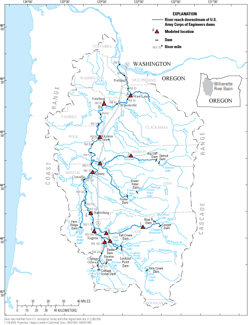
Willamette River network, locations of major dams, and sites for which temperature regression models were developed, northwestern Oregon. Map adapted from Rounds (2010). Letters correspond to the modeled locations in tables 1 and 2. (A) Willamette River at river mile 26.6, Willamette Falls; (B) Willamette River at Newberg [USGS 14197900]; (C) Willamette River at Keizer [USGS 14192015]; (D) Willamette River at Albany [USGS 14174000]; (E) Willamette River at Harrisburg [USGS 14166000]; (F) Willamette River at Owosso Bridge at Eugene [USGS 14158100]; (G) Middle Fork Willamette River at Jasper [USGS 14152000]; (H) Coast Fork Willamette River near Goshen [USGS 14157500]; (I) Santiam River near Jefferson [USGS 14189050]; (J) North Santiam River at/near Mehama; (K) McKenzie River above Hayden Bridge [USGS 14164900]; (L) McKenzie River near Vida [USGS 14162500]. North Santiam River at/near Mehama is a spliced record created after the continuous temperature monitor was moved slightly downstream in order to remove the effects of unmixed water incoming from Little North Santiam River.
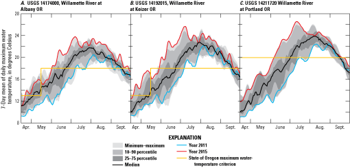
Measured water temperatures in the Willamette River at (A) USGS site 14174000 at Albany, (B) USGS site 14192015 at Keizer, and (C) USGS site 14211720 at Portland, northwestern Oregon.
The Willamette Valley Project is a system of 13 dams, numerous revetments, and several fish hatcheries in the Willamette River basin owned by the USACE. It is operated to minimize the risk of downstream floods, generate electrical power, provide recreational opportunities, and augment summertime streamflow for navigation and fish habitat, among other purposes. Current summer minimum streamflow targets in the Willamette River at Albany and Salem are higher than pre-dam summer streamflows by about a factor of two (Rounds, 2010; U.S. Geological Survey, 2019). Originally authorized in 1938 to provide summer navigation upstream of Willamette Falls and for the “beneficial effect on fish life” of the Willamette River’s then heavily polluted waters, minimum streamflow targets were formalized for the benefit of threatened fish populations in the 2008 Biological Opinion (National Marine Fisheries Service, 2008) and have been increasingly recognized as beneficial for improving habitat conditions, including water temperature. Flow augmentation decreases summer stream temperatures in the Willamette River by increasing the river’s “thermal mass” (which buffers its temperature response to incoming heat fluxes), decreasing the travel time from cooler headwater locations and typically decreasing the width-to-depth ratio of the Willamette River (Rounds, 2007; Risley and others, 2010). However, the potential for flow management actions to directly affect stream temperature in downstream reaches is poorly understood, and linkages between the effects of flow management and the recovery of threatened fish populations remain difficult to characterize.
To better understand the thermal dynamics of the Willamette River and its tributaries downstream of USACE dams and to inform how flow management actions in the Willamette River basin can support both native resident fish and threatened anadromous fish, USACE asked the United States Geological Survey (USGS) to develop a set of computational tools for evaluating the influence of streamflow on stream temperature in the Willamette River system. Deterministic stream temperature modeling that accounts for the full suite of influential heat fluxes and environmental variables across a range of climatic conditions has been performed in the Willamette River basin in the past (for example, Rounds, 2010). The use of deterministic models, however, is data and computation intensive and impractical for many management applications. In contrast, statistics-based approaches provide reasonable estimates of stream temperature based on relatively simple mathematical relations (Mohseni and others, 1998; Donato, 2002; Neumann and others, 2003; Isaak and others, 2017). Regression models can be easily incorporated into sophisticated reservoir-operation or flow-optimization models because regression models tend to have a small number of inputs, are often based on relatively simple equations, and are not computationally demanding to solve or implement.
In this study, regression relations were developed to predict the 7-day average of the daily mean (7dADMean) and the 7-day average of the daily maximum (7dADMax) water temperature at 12 stream sites in the Willamette River basin and were applied to improve understanding of the thermal response of the rivers to changes in streamflow and air temperature. Water-temperature models were built using publicly available air temperature, streamflow, and stream temperature data. Seasonality in the relation between water temperature and streamflow was addressed by breaking the year into different seasons and building optimized multiple linear regression models for each season. The resulting relations provide simple tools to investigate the response of stream temperature to changes in streamflow and provide general insights into how the Willamette River system responds to the effects of streamflow and weather conditions.
Description of Study Area
The Willamette River drains approximately 11,500 square miles (mi2) of northwestern Oregon between the Coast Range and the Cascade Range, flowing for 187 miles (mi) from its start at the confluence of the Middle and Coast Forks of the Willamette River, south of Eugene, to its confluence with the Columbia River near Portland (fig. 1). Flow in the Willamette River is predominantly confined to a single, main channel, but side channels, alcoves, and other secondary channel features intermittently flank the main channel and are most common between Eugene and Corvallis (Gregory and others, 2002; Wallick and others, 2013). The basin has a maritime climate with cool, wet winters, and dry summers. Winter storms typically track from the Pacific Ocean eastward, dropping the majority of precipitation as rain in the Coast Range and valley bottom and as rain and snow in the Cascade Range. Average precipitation in the basin ranges from 1,000 millimeters per year (mm/yr) in the valley to as much as 2,600 mm/yr along the Cascade Crest (PRISM Climate Group, 2020).
Streamflow and temperature in the Willamette River and its tributaries are influenced by the prevailing climate, variations in the weather, the geology and topography of the basin, riparian vegetation, and the timing and volume of dam releases, among other factors. Tributaries draining the Coast Range are rain-dominated and generally drain relatively impermeable bedrock; as a result, summer baseflow is low and stream temperatures tend to be relatively high (Conlon and others, 2005; Dent and others, 2008; Bladon and others, 2018). The topography and hydrology of the Cascade Range is dominated by the Western Cascades, composed of deeply dissected, relatively impermeable volcanics that tend to occur at moderate elevations, and the High Cascades, composed of young, highly permeable, high-elevation volcanic plateaus (Ingebritsen and others, 1994; Conlon and others, 2005; Jefferson and others, 2006). Tributary flow originating in the Western Cascades tends to closely follow seasonal precipitation and temperature patterns and is dominated by shallow subsurface runoff derived from rain events. In contrast, tributaries originating in the High Cascades are dominated by groundwater from snowmelt-fed springs and thus tend to exhibit more-stable streamflow and colder, more-stable temperature patterns (Tague and Grant, 2004; Tague and others, 2007). Groundwater contributions to High Cascade-sourced tributaries comprise a large part of flow in the Willamette River, particularly during the low-flow season.
The Willamette River basin historically supported populations of salmon and steelhead across much of the basin, but USACE dams block upstream migrants from accessing an important part of their historical spawning grounds, and the dams and revetments of the USACE Willamette Valley Project affect flow, fish habitat, and temperature conditions along river reaches that historically provided the primary spawning, migration, and rearing corridors for spring Chinook salmon upstream of Willamette Falls. In 2008, the National Marine Fisheries Service (NMFS) determined that continued operation of the dams would jeopardize the sustainability of protected anadromous fish species (National Marine Fisheries Service, 2008). This jeopardy determination resulted in the mandate of a series of remediation actions, including management to restore temperatures downstream of dams to a more natural thermal regime, establishment of fish passage at the dams, formalization of flow and temperature targets in the Willamette River at Albany and Salem, and research to better understand the needs of anadromous fish species. Since 2008, thermal regimes in some river reaches have improved because of adjustments to flow management and alterations to the structural outlets and operations at USACE dams (Rounds, 2007; Rounds, 2010; Hansen and others, 2017). Barriers to fish passage, detrimentally high temperatures in the downstream reaches of the Willamette River, and altered thermal regimes downstream of multiple dams, however, are still areas of concern and active research and management.
Purpose and Scope
This report documents the development of regression-based tools to estimate stream temperature in the Willamette River and its major tributaries and the use of those predictions to (1) better understand the range of stream temperatures anticipated under historical climatic and streamflow conditions and (2) investigate the potential for flow management to influence stream temperature.
Regression models documented in this report focus on the main stem and sub-basins of the Willamette River basin with formerly abundant anadromous fish populations affected by USACE dams, including the North and South Santiam River sub-basins, the McKenzie River sub-basin, and the Middle Fork and Coast Fork Willamette River sub-basins (National Marine Fisheries Service, 2008; Hansen and others, 2017). The regression models predict stream temperature near USGS or other continuous data collection sites located in the main channels of the Willamette, North Santiam, South Santiam, Santiam, McKenzie, Coast Fork Willamette, and Middle Fork Willamette Rivers. Regression models utilized water temperature, air temperature, and streamflow data collected from 2000 to 2018; data at a few sites were restricted to more-recent years to ensure consistency with changes to upstream dam operations that occurred in 2005 (McKenzie River) and 2007 (North Santiam River). Use of the models to analyze the effects of climatic variability and flow management were restricted to several key sites along the Willamette River (Harrisburg, Albany, and Salem/Keizer). The effects of flow alterations were analyzed by incrementally increasing or decreasing modeled streamflow by a maximum of 1,000 ft3/s relative to measured streamflows in 2018. The report includes a discussion of the limitations of the models and their application; however, generally, these models provide an easily applied, relatively accurate, and computationally efficient estimate of stream temperature when the application of more detailed, process-based models may not be practical or when there is a need to identify scenarios and conditions that warrant more evaluation from process-based models.
Definitions and Terms Used in this Report
This report uses a variety of terms to describe stream temperature conditions across different seasons and climatic scenarios. To the extent possible, the following set of terms and climatic scenarios are applied systematically across the report:
-
• Seasons are defined according to the boundaries of the seasonal regression models included in the smoothed, piecewise annual regression:
-
• Year types are defined according to the air temperature and streamflow quantiles across the period of analysis (1954–2018). “Much below” and “much above” normal (very cool or dry or very warm or wet) are defined as the 0.10- and 0.90-quantiles of the data; “below” and “above” normal (cool or dry or warm or wet) are defined as the 0.33- and 0.67-quantiles of the data; “normal” represents the median (0.50-quantile) (National Centers for Environmental Information [NCEI], 2020). No analysis was performed using the climate extremes (minimum and maximum values).
When used in reference to an annual synthetic time series, year type refers to a time series comprised of daily values representing the extreme of quantile range (for example, in a “very cool and very wet” year, the data are comprised of the 0.10 quantile of air temperature and the 0.90 quantile of streamflow for the calendar day in question from 1954 to 2018). While the period of record for both air temperature and streamflow at many sites extends prior to 1954, those data were censored to exclude data before the implementation of summer flow augmentation by Willamette Valley Project dam releases, most of which had been built and were operating by 1954.
When used in reference to a specific year or season, the year type indicates that the record in question falls within the defined quantile range; for example, streamflow at Salem in summer 2016 was “below normal,” indicating that, on average, it was within the 0.33–0.50 quantile range for June, July, and August during 1954–2018.
Methods and Models
Model Development
Regression models quantify the relation between one or more explanatory variables and a response variable by fitting an equation to the observed data such that error in the resulting model is minimized. Approaches vary from simple linear regression, which fits a linear model between a single explanatory response pair, to more sophisticated methods utilizing multiple explanatory variables, piecewise approaches, or nonlinear methods. When developing a good regression model, a priori understanding of controlling processes can help the modeler select appropriate explanatory variables and determine the nature of their relation to response variables.
Because the largest fluxes of heat to and from a stream typically occur across the air/water interface, air temperature and stream temperature tend to be closely correlated, and the strength of that correlation tends to increase with increasing travel time (distance) downstream from other influencing factors such as tributary inputs, point sources, or dams. Consequently, air temperature has been widely used to approximate stream temperature with generally good accuracy at weekly or monthly timescales, using both linear and logistic regression equations (Johnson, 1971; Mohseni and others, 1998; see also, Caissie, 2006).
Stream temperature, however, is not solely a function of heat flux inputs, for which air temperature often is used as a surrogate. Instead, stream temperature is analogous to the heat content or “heat concentration” in a system, where changes in water temperature are known to be a function of the change in heat content, the mass of water undergoing the temperature change, and the specific heat of water. Using air temperature as a surrogate for environmental heat fluxes (such as short-wavelength solar radiation and long-wavelength atmospheric radiation) and changes in heat content and using streamflow as a surrogate for the mass of water and the time available for heat fluxes to occur, it is reasonable that the temperature of a stream should be proportional to air temperature and streamflow. A more detailed discussion of these concepts has been published by Brown (1969), Poole and Berman (2001), and Caissie (2006). The resulting function can be written as:
whereThe dependence of water temperature on the reciprocal of streamflow is consistent with the fact that increases in streamflow would decrease the time available for environmental heat fluxes to warm or cool the water and would increase the mass of water in the stream to resist any changes in temperature. Both effects suggest that changes in water temperature would decrease as streamflow increases, a relation that is embodied in the reciprocal transformation to 1/Q required to linearize the relation between stream temperature and streamflow.
Maximum temperature criteria in the State of Oregon water-temperature standard are defined based on the 7-day average of the daily maximum (7dADMax; Oregon Department of Environmental Quality, 2020). At this time scale, the relation between air temperature and stream temperature in the Willamette River system can be reasonably approximated as linear (fig. 3); however, some seasonal hysteresis1 is evident. In addition, at the extremes of the temperature range, the relation appears to “level off,” suggesting that stream temperature may be better approximated by a sigmoid (or logistic) function. Relations between air temperature and stream temperature for the 7dADMean show similar patterns (fig. 4). Scatter plots relating the 7dADMean of the reciprocal of streamflow (1/Q) to the 7dADMean or 7dADMax stream temperature also show some definite relations; however, these relations are more complicated than that of air temperature with stream temperature. During spring, summer, and autumn, the relation between 1/Q and stream temperature, while exhibiting substantial scatter, is reasonably curvilinear (figs. 5–6). From December through the winter, however, stream temperature appears to be relatively independent of the magnitude of streamflow, as indicated by the scatter in the plotted relations.
Hysteresis is a term indicating that the warming trajectory from winter to summer on a graph of water temperature versus air temperature may take a slightly different path than the cooling trajectory from summer to winter; such hysteresis may be indicative of time lags in the seasonal heating and cooling of the rivers (Mohseni and others, 1998, 199921).
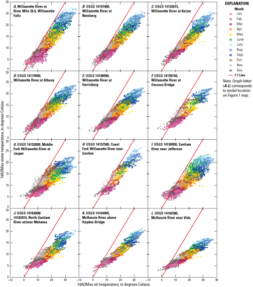
Relations between the measured 7-day average of the daily maximum (7dADMax) air temperature and the measured 7dADMax water temperature at 12 sites for which water-temperature regression models were developed, Willamette River basin, northwestern Oregon.
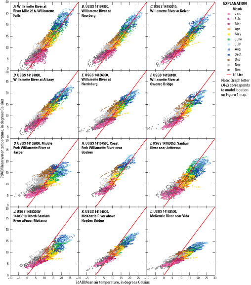
Relations between the measured 7-day average of the daily mean (7dADMean) air temperature and the measured 7dADMean water temperature at 12 sites for which water-temperature regression models were developed, Willamette River basin, northwestern Oregon.
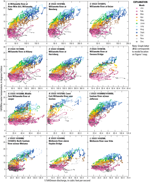
Relations between the measured 7-day average of the daily mean (7dADMean) of the reciprocal of streamflow and the 7-day average of the daily maximum (7dADMax) water temperature at 12 sites for which water-temperature regression models were developed, Willamette River basin, northwestern Oregon.
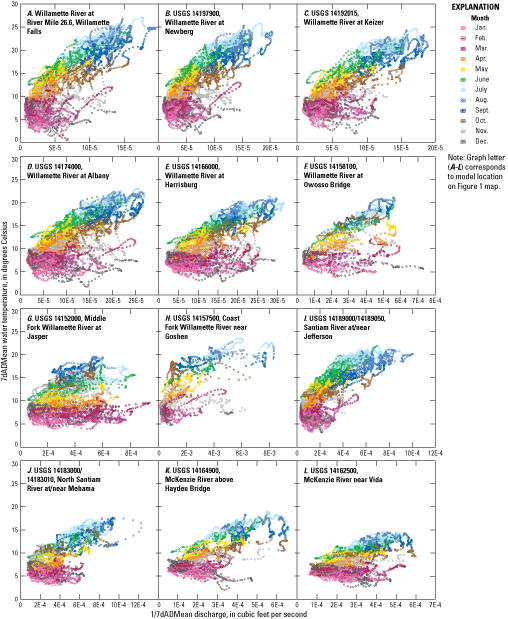
Relations between the measured 7-day average of the daily maximum (7dADMean) of the reciprocal of streamflow and the measured 7dADMean of water temperature at 12 sites for which water-temperature regression models were developed, Willamette River basin, northwestern Oregon.
To account for the seasonal differences in the relations between water temperature, air temperature, and particularly streamflow, a piece-wise approach to model development was applied. By separating each year into five distinct time periods (or “seasons”) according to natural breakpoints in the relations among water temperature, air temperature, and streamflow, stream temperature within each time period can be reasonably approximated using a multiple linear regression approach, where:
wheres
is the seasonal time-period index,
is the estimated 7-day average daily mean or maximum stream temperature, in degrees Celsius,
is the 7-day average mean or maximum air temperature, in degrees Celsius,
Q
is the 7-day average streamflow, in cubic feet per second,
are regression coefficients, and
is the regression intercept.
Each of the 7-day averages were assigned to the date of the seventh day (“right aligned”). Different seasonal breakpoints and numbers of seasonal models were evaluated to optimize the annual model. Based on this optimization analysis, the final time periods for the seasonal model indices (s) were chosen to be: Winter: Day of year 1–90 (January 1st–March 31st),Spring: Day of year 91–151 (April 1st–May 31st),Summer: Day of year 152–243 (June 1st–August 31st),Early autumn: Day of year 244–304 (September 1st–October 31st), andAutumn: Day of year 305–365 (November 1st–December 31st).
This piecewise approach of using seasonal models can create undesirable discontinuities in predicted stream temperature at date boundaries of adjacent seasonal models. To address this problem, logistic functions were used as multipliers to smooth the transitions between seasonal regression model predictions, as follows:
whereis the transition multiplier function at day JDAY for seasonal models,
e
is the natural logarithm base,
k
is the steepness of the transition curve (a value of 1 was used),
JDAY
is the day of year,
is the lower date boundary for seasonal model s, expressed as a day of year (values 0.5, 90.5, 151.5, 243.5, 304.5), and
is the upper date boundary for seasonal model s, or the lower date boundary for seasonal model s+1, expressed as a day of year (values: 90.5, 151.5, 243.5, 304.5, 365.5).
When the JDAY of interest is between and substantially away from the boundary dates for a seasonal model, both terms in equation 3 are near or equal to 1.0 and the overall multiplier for that seasonal model is essentially 1.0. When JDAY is outside the lower and upper date boundaries of one of the five seasonal models, one of the terms diminishes toward 0.0, and therefore the multiplier is nearly 0.0 and the influence of that seasonal model is eliminated for periods outside of its date range.
When making predictions near the beginning or end of the year, the final temperature prediction must account for transitions across the year boundary, from the autumn model of the previous year to the winter model of the current year and from the autumn model of the current year to the winter model of the next year. To incorporate these transitions, multipliers from autumn of the previous year (JDAY +365) and for winter of the following year (JDAY – 365) must be calculated. Incorporating those transitions and combining equations 2 and 3, a final estimate of 7dADMean or 7dADMax stream temperature can be calculated as:
whereis the 7-day average mean or maximum stream temperature on any day of the year that accounts for all five seasonal models and the transitions between them,
is the 7-day average mean or maximum stream temperature for each seasonal model as estimated by equation 2, and
is the season- and JDAY-specific multiplier as defined in equation 3.
The next-to-last term in equation 4 accounts for the influence of the autumn model (season 5) on JDAYs less than 5 or so, and the last term provides the influence of the winter model (season 1) on JDAYs near the end of the current year.
Data Sources and Processing
Regression models of the 7dADMean and 7dADMax stream temperature were developed for 12 locations in the Willamette River and key tributaries (fig. 1), as described in, “Model Development,” above. Seasonal breaks were defined uniformly across the river network. All regression calculations were based on calendar day of year (JDAY); a sensitivity analysis indicated that leap years could be ignored (discarding day 366) when assigning JDAY to calendar dates without a meaningful difference in the resulting goodness-of-fit statistics. Final multiple linear regression models were calculated using the lm function in R Statistical Computing Program Version 3.5.2, “Eggshell Igloo” (R Core Team, 2018). The lm function applies a least-squares method to estimate regression fits, following the methodology of Wilkinson and Rogers (1973) and Chambers (1992). Season-specific regression coefficients and goodness-of-fit metrics are included in tables 1.1–1.12 of appendix 1. Source data, models, goodness-of-fit statistics, seasonal break definitions, the logistic multiplier function, and supporting plotting, prediction, and scenario analysis R scripts have been archived and are available from USGS Science Base (Stratton Garvin, 2021).
The development of each regression model required three datasets as inputs: (1) 7dADMean or 7dADMax air temperature, (2) 7dADMean or 7dADMax stream temperature, and (3) 7dADMean streamflow. Air temperature, streamflow, and stream temperature data for the 7dADMean and 7dADMax stream temperature models were obtained from several sources, including the National Oceanic and Atmospheric Administration (NOAA), USGS, Portland General Electric (PGE), and USACE, as detailed in table 1. For ease of use when connecting these regression models with other tools and models, the regression models employed mixed unit systems. All streamflow data were measured and used in cubic feet per second, and all air- and water-temperature measurements and estimates were applied in the models in degrees Celsius.
Table 1.
Site locations, river miles, data sources, and length of record for datasets used in the 12 water-temperature regression models developed at key sites in the Willamette River system, northwestern Oregon.[River miles are presented as reported by U.S. Geological Survey (USGS) National Water Information System water-year summaries where available; otherwise they are presented as measured from USGS digital topographic maps. Each river mile is measured from its downstream confluence; for example, the Willamette River is measured from its confluence with the Columbia River. The Middle Fork Willamette uses Willamette River miles. The Coast Fork Willamette River is measured from its confluence with the Middle Fork Willamette River. Calibration period format is month-day-year. Abbreviations: ODFW, Oregon Department of Fish and Wildlife; USACE, U.S. Army Corps of Engineers; USGS, U.S. Geological Survey; WBAN, Weather-Bureau-Army-Navy site identifier]
To allow application in a real-time situation, all relations were based on right-aligned 7-day moving averages (the average of the day in question and the 6 days prior) of the daily mean or maximum derived from measured daily or subdaily data, except for the Willamette Falls site (RM 26.6), which required estimation of several data inputs. Streamflow at Willamette Falls was estimated as the sum of the streamflows measured at USGS streamgages on the Willamette River at Newberg (USGS site 14197900), the Pudding River at Aurora (USGS site 14202000), the Mollala River near Canby (USGS site 14200000), and the Tualatin River at West Linn (USGS site 14207500; table 1). These streamgages account for 97.6 percent of the drainage area to the Willamette River at Willamette Falls but do not capture small volumes of ungaged sources, particularly from small creeks and overland flow during storms. Stream temperature data at Willamette Falls were collected by the Oregon Department of Fish and Wildlife (ODFW) at the Willamette Falls fish ladder from a fixed, enclosed thermometer marked in 2-degree Fahrenheit gradations. Readings were collected manually once daily, generally on workdays (excluding weekends and holidays) about 7:30 a.m. (Kevleen Melcher, Oregon Department of Fish and Wildlife, personal communication, 2020). To produce the time series used in this report, ODFW data were compared to daily mean temperatures from Newberg (USGS 14197900) to produce an estimate of daily mean temperature at Willamette Falls:
whereis the mean daily water temperature at Willamette Falls in degrees Celsius, and
is the mean daily water temperature at USGS site 14197900, Willamette River at Newberg, in degrees Celsius.
The 7dADMax stream temperature at Willamette Falls was estimated as:
whereis the daily maximum water temperature at Willamette Falls in degrees Celsius,
is the constructed daily mean water temperature from equation 5 at Willamette Falls in degrees Celsius,
is the daily maximum water temperature at USGS site 14197900, Willamette River at Newberg, in degrees Celsius, and
is the daily mean water temperature at USGS site 14197900, Willamette River at Newberg, in degrees Celsius.
The temperature estimates produced using equations 5 and 6 were compared to a continuous temperature dataset from USGS 14207740 (Willamette River above Willamette Falls), available for discontinuous periods from 2001 to 2003, to verify that no bias was introduced by using the morning temperature data collected by ODFW. Estimates of the 7dADMean and 7dADMax stream temperature at Willamette Falls produced using a simple linear regression with the USGS data yielded R2 values of 0.99 (7dADMean and 7dADMax) and a mean error (a measure of model bias) of less than 0.1°C for both datasets. This relation indicates that both the 7dADMean and 7dADMax stream temperature at Willamette Falls, as estimated using equations 5 and 6, are reasonable approximations. Air temperature data for the Willamette Falls model were sourced from measurements collected at the Salem, Oregon airport (WBAN site 24232; table 1), which resulted in a more accurate model compared to one based on air-temperature data from the Portland International Airport.
Regression relations for the North Santiam River near Mehama were based on water-temperature data collected at USGS site 14183000 (North Santiam River at Mehama) from 2007 to 2009 and at USGS site 14183010 (North Santiam River near Mehama) from 2009 to 2015, according to the availability of temperature data. The site for temperature data collection was moved from site 14183000 to site 14183010 in October 2009 after it was recognized that site 14183000 was too close to the upstream confluence of the Little North Santiam River with the North Santiam River and that water-temperature measurements at site 14183000 were more representative of the Little North Santiam River when Little North Santiam River flows were high (particularly in spring). Both were included here to increase the length of record available. Temperature data collected at site 14183000 prior to 2007 were excluded from this analysis because operations at Detroit Dam upstream were different prior to 2007, and the pre-2007 operations resulted in water temperatures that had a different seasonal pattern.
Streamflow and stream temperature data, in many cases, were collected from measurement sites that were adjacent but not co-located. The stream temperature model for the Willamette River in Eugene is based on water temperature data from USGS site 14158100 (Willamette River at Owosso Bridge, river mile [RM] 178.8), whereas the streamflow data are from USACE streamgage EUGO3 (as of 2016, synonymous with USGS streamgage 14158050, Willamette River at Eugene; RM 184.5), approximately 6 mi upstream. Similarly, the stream temperature model for the Willamette River at Keizer is based on water temperature data from USGS site 14192015 (Willamette River at Keizer, RM 82.2), whereas the streamflow data are from USGS site 14191000 (Willamette River at Salem, RM 84.0). Finally, the temperature model for the Santiam River near Jefferson uses streamflow data from a streamgage located 3.4 mi upstream. The strength of these relations depends on the absence of significant flow inputs between the streamflow and stream temperature measurement sites, which appears to be a reasonable assumption in each of these cases. River mile designations used in this report are as reported by NWIS water-year summaries (U.S. Geological Survey, 2019); where no river mile is reported for a site or streamgage, river miles were estimated from USGS topographic maps.
Although air temperature and streamflow data in the Willamette Valley are available from the 1940s or earlier (for example, USGS streamflow data are available as early as the 1890s at the Albany streamgage) and daily stream temperature data may be available from USGS from the 1970s or 1980s (U.S. Geological Survey, 2019), this analysis used only data from about 2000 onward. Restricting model inputs to a more-recent time period serves multiple purposes. First, a more-recent time period coincides with the widespread availability of reliable and accurate (±0.2 °C) sensors to collect subdaily temperature data. Second, the use of more-recent data limits the effect of any long-term trends in air temperature and in the relation between air temperature and streamflow or dam operations. These “modern” models, therefore, do not and cannot account for any long-term effects such as the evolution of river shading, surface and subsurface flow paths, channel complexity and other geomorphic features, or trends in streamflow. This limits the use of the models, without extrapolation, to the range of data inputs for 2000–2018 and requires an assumption of approximately “modern” river characteristics (see “Discussion–Model Limitations” section for more discussion).
Model Evaluation
Seasonal boundaries and regression models were developed iteratively to minimize model bias and error and were subjected to standard regression evaluation measures. Confidence in the final fit of the regression models was calculated using three metrics: the mean error (ME; eq. 7), the mean absolute error (MAE; eq. 8), and the root mean square error (RMSE; eq. 9), with a focus on the latter two.
whereis the model-estimated temperature, in degrees Celsius,
is the observed temperature, in degrees Celsius, and
n
is the number of data points.
The ME is a measure of model bias. The MAE is an estimate of the magnitude of the typical average prediction error of the model. The RMSE is essentially the standard deviation of the error distribution; therefore, if the model errors follow a normal distribution, about two-thirds of the errors would be smaller than the RMSE and about 95 percent of the model errors would be smaller in magnitude than twice the RMSE. Because the errors are squared prior to averaging, RMSE tends to give higher weight to large errors than does the MAE.
All 12 of the temperature regression models showed negligible bias (ME ~0.0 °C) and resulted in annual MAE ≤1.0 °C and RMSE ≤1.2 °C, and often less, at many locations (table 2; figs. 7–8). The models for the Willamette Falls site showed relatively poor performance, despite the location of the site well downstream of any upstream dams; the higher model error likely is attributable to higher uncertainty in the streamflow and water-temperature data used as input to those models. Sensitivity testing showed that the steepness of the logistic curve used to smooth seasonal models (k in equation 3) did not have an important effect on model error. A value of 1 was used for k in the final model.
Table 2.
Goodness-of-fit statistics for the 7-day average of the daily mean (7dADMean) and 7-day average of the daily maximum (7dADMax) stream temperature at 12 modeled locations in the Willamette River stream network, northwestern Oregon.[Abbreviations: ME, mean error; MAE, mean absolute error; RMSE, root mean square error; °C, degrees Celsius]
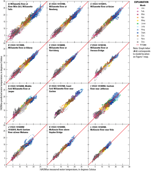
Comparison of measured and predicted 7-day average of the daily maximum (7dADMax) water temperature at 12 sites for which water-temperature regression models were developed, Willamette River basin, northwestern Oregon. A 1:1 line is shown for comparison; a perfect fit would have all points fall on the 1:1 line. Colors indicate the month of the year. Letters correspond to map locations on figure 1.
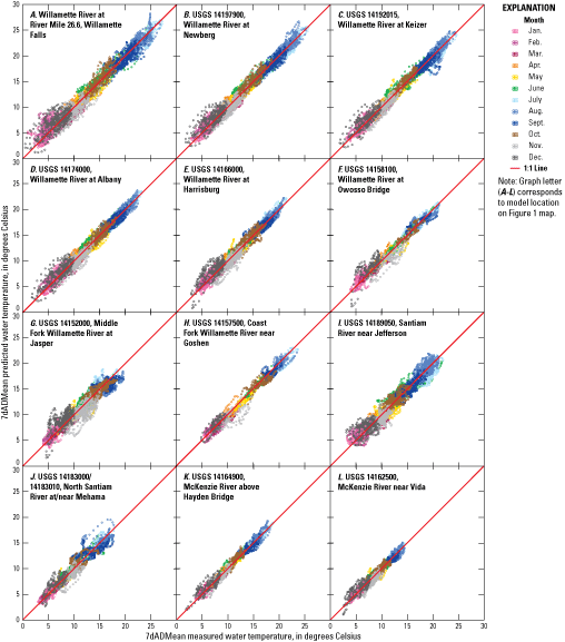
Comparison of measured and predicted 7-day average of the daily mean (7dADMean) water temperature at 12 sites for which water-temperature regression models were developed, Willamette River basin, northwestern Oregon. A 1:1 line is shown for comparison; a perfect fit would have all points fall on the 1:1 line. Colors indicate the month of the year. Letters correspond to map locations on figure 1.
Willamette River Temperature Regimes
Climatological Analysis of Predicted Temperature
By modeling stream temperature across a broad range of air temperature and streamflow conditions, the models developed in this study can be used to better understand the thermal regimes of the Willamette River system and how stream temperature response to flow management varies across the stream network. Using these models, estimates of stream temperatures at Harrisburg, Albany, and Keizer were predicted using annual synthetic time series representing the 0.10, 0.33, 0.50, 0.67, and 0.90 quantiles of the air temperature and streamflow distributions for each day of the year. The quantile distributions were based on measured data from 1954 to 2018, which was after the construction of many of the large dams of the Willamette Valley Project. These quantiles correspond to the NCEI climatological rankings for a “normal” (median), “below or above normal” (0.33 or 0.67 quantiles), or “much below or much above normal” (0.10 or 0.90 quantiles) year (NCEI, 2019). Any predicted stream temperatures below zero (limited to January in scenarios “much below normal” for air temperature) were replaced with zero. Not all conditions would be expected to co-occur naturally with the same frequency; additionally, no year is composed entirely of days falling into a single quartile. For example, while June in a single year may be of “normal” air temperature and “above normal” streamflow, November of the same year may have “much above normal” air temperatures and “much above normal” streamflows. Furthermore, by excluding the minimum and maximum air temperature and streamflow records from the analysis described in this section, extremes are not considered. By examining the stream temperature response to air temperature and streamflow conditions ranging from “much-below to much-above” normal (0.1–0.9 quantiles), however, valuable insights can be gained into the range of possible stream temperatures in the Willamette River basin.
According to the form of the regression models, cool stream temperatures would be expected from a combination of cool air temperatures and high streamflows, whereas high stream temperatures would be anticipated from a combination of warm air temperatures and low streamflows. Thus, to define the lower range of anticipated stream temperatures in the Willamette River (excluding extreme conditions beyond the range of reasonable model prediction), estimates of stream temperature were calculated using time-series inputs from the 0.10 quantile of air temperature combined with the 0.90 quantile of streamflow for each day to create a synthetic “very cool, very wet year.” Conversely, the upper range of anticipated stream temperatures was calculated using time-series inputs from the 0.90 quantile of air temperature and the 0.10 quantile of streamflow to represent a “very hot, very dry year.”
Summer water temperatures predicted across the range of climate scenarios imposed from Harrisburg to Keizer resulted in 7dADMax ranges of about 3 to over 5 °C, depending on location (fig. 9). Mean July 7dADMax under “normal” (median) air temperature and streamflow conditions ranged from 20.9 °C at Keizer to 18.7 °C at Harrisburg (table 3). At Harrisburg, predicted mean June 7dADMax temperatures range from 13.4 °C in very cool and very wet conditions to 18.8 °C in very hot and very dry conditions, a difference of 5.4 °C. In July, mean 7dADMax modeled temperatures increase to 16.7 °C for very cool and very wet conditions and 20.8 °C for very hot and very dry conditions, with a similar range of 16.9 to 20.4 °C in August (table 3; fig. 9). At Albany and Keizer, the range of modeled 7dADMax water temperatures across these climate scenarios increases, probably reflecting greater variance in summer streamflow between a very dry and very wet year, in addition to having more time for the river to warm during hot periods as the water moves downstream. In July and August in very hot and very dry years, monthly mean 7dADMax temperatures are predicted to exceed 22.1 °C at Albany and 23.7 °C at Keizer, whereas in very cool and very wet years, July and August monthly average 7dADMax temperatures are predicted to range from 17.8 to 19.1 °C at Albany and Keizer (table 3).
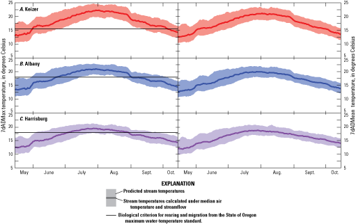
Predicted 7-day average of the daily maximum (7dADMax) and 7-day average of the daily mean (7dADMean) water temperature from regression models using a range of 7dADMean streamflow and 7dADMax or 7dADMean air-temperature conditions to define a range of water temperatures for (A) Keizer, (B) Albany, and (C) Harrisburg along the Willamette River, northwestern Oregon. The shade ribbons indicate predicted stream temperatures calculated using 0.90 and 0.10 air temperature and streamflow (very hot and very dry) and 0.10 and 0.90 air temperature and streamflow quantiles (very cool and very wet). The air temperature and streamflow quantiles were based on data from 1954 to 2018.
Table 3.
Monthly means of the predicted 7-day average of the daily maximum (7dADMax) stream temperature using a range of streamflow and air-temperature conditions for three sites in the Willamette River, northwestern Oregon.[“Much below” and “much above” normal are defined as the 0.10- and 0.90-quantiles of the data; “below” and “above” normal are defined as the 0.33- and 0.67-quantiles of the data; “normal” represents the median (0.50-quantile). The air temperature and streamflow quantiles were based on data from 1954 to 2018]
Summer 7dADMean stream temperatures under median air temperature and streamflow conditions warm through early summer before peaking in late July or early August and cooling through September (fig. 9). At Keizer, the median (“normal”) predicted 7dADMean stream temperature for the month of June under median streamflow and air temperature conditions is 16.4 °C, increasing to 19.9 °C in July and 20.5 °C in August (table 4). These monthly means, however, may vary by more than 5 °C from a very cool, very wet year to a very dry, very hot year. For example, the mean June temperature in a very cool, very wet year is predicted to be 14.0 °C at Keizer, while in a very hot, very dry year, it is predicted to be 19.5 °C (table 4). The temperature range at Albany and Harrisburg, upstream, is slightly greater, with a difference of up to 5.5 °C between a very cool, very wet year and a very dry, very hot year at Harrisburg in June (table 4). In a median streamflow, median air-temperature year, mean 7dADMean temperatures at Albany are >19 °C in July and August, while at Harrisburg, mean 7dADMean temperatures in July and August are close to 18 °C. The range of predicted temperatures across air temperature/streamflow scenarios decreases from June through August, with the difference in predicted temperatures between a very cool, very wet year and a very hot, very dry year only 3.5 °C in August at Harrisburg. This variation in the range of predicted temperatures probably reflects a similar decrease in the range of streamflow variation with the progression of the summer dry period.
Table 4.
Monthly means of the predicted 7-day average of the daily mean (7dADMean) stream temperature using a range of streamflow and air-temperature conditions for three sites in the Willamette River, northwestern Oregon.[“Much below” and “much above” normal are defined as the 0.10- and 0.90-quantiles of the data; “below” and “above” normal are defined as the 0.33- and 0.67-quantiles of the data; “normal” represents the median (0.50-quantile). The air temperature and streamflow quantiles were based on data from 1954 to 2018]
Model results indicate that, except in cool and very wet years, the Willamette River is likely to exceed the State of Oregon maximum water-temperature standard for sustained periods during summer from Newberg to Harrisburg, and possibly farther upstream. The regulatory criteria for temperature in the Willamette River upstream of Newberg are 18 °C (to protect rearing and migration fish uses; measured as the 7dADMax) for May 16th to October 14th, and 13 °C (to protect spawning fish use) for the remainder of the year (Oregon Department of Environmental Quality, 2003, 2005, and 2020). Model results indicate that, under the range of climate scenarios modeled, the 7dADMax water temperature in the Willamette River is predicted to exceed 18 °C as far upstream as Harrisburg for much of the summer (fig. 9); however, the duration and degree of exceedance varies by location. In a very hot and very dry year, the 7dADMax Willamette River temperature at Keizer is predicted to exceed 18 °C for as many as 133 days, whereas the number of exceedance days at Harrisburg may be as many as 110 (table 5). The number of exceedance days decrease progressively across cooler, wetter climate scenarios; however, in a very cool and very wet year, 7dADMax temperatures are still predicted to remain above 18 °C for 38 days as far upstream as Albany, and the 7dADMax temperature at Harrisburg is expected to remain at or slightly below 18 °C for the duration of summer (table 5; fig. 9).
Table 5.
Number of days that the predicted 7-day average of the daily maximum (7dADMax) water temperature at Keizer, Albany, and Harrisburg exceeds 18 degrees Celsius as calculated from designated climate scenarios, Willamette River, northwestern Oregon.[“Much below” and “much above” normal are defined as the 0.10- and 0.90-quantiles of the data; “below” and “above” normal are defined as the 0.33- and 0.67-quantiles of the data; “normal” represents the median (0.50-quantile). The air temperature and streamflow quantiles were based on data from 1954 to 2018]
Temperature Sensitivity to Flow Management: 2018
In addition to bracketing the range of temperature variation across potential climate scenarios at sites in the Willamette River system, the regression models can provide an estimate of temperature sensitivity to specific flow management strategies. Summer 2018 can be used as an interesting example. NCEI ranked the 3-month average air temperature from June to August 2018 in the Willamette Valley as 7 out of 126 (1895–2019), or “much-above normal” (NCEI, 2020). Using the same approach, the average streamflow at Salem (USGS 14191000) from June through September of 2018 ranks 21 of 67 (1954–2020), near the “below normal”/“near normal” threshold (22) (U.S. Geological Survey, 2019). Summer 2018, therefore, might be classified as very hot with near to below-normal streamflow. Predictions of mean monthly 7dADMax stream temperature from the regression models using 2018 inputs indicate that at modeled streamflows that are ±100 to ± 1,000 ft3/s different from measured values, stream temperatures at Harrisburg, Albany, and Keizer could change by as little as <0.1°C or by as much as 1.4 °C in June, July, and August (table 6) and that the influence of flow management varies by location, month, and the direction of flow management (increase or decrease).
Table 6.
Predicted differences in the monthly mean of the 7-day average of the daily maximum (7dADMax) water temperature and the change in the number of days in exceedance of the water quality standard at Keizer, Albany, and Harrisburg, Willamette River, northwestern Oregon.[Predictions use the regressions models for each site, applying measured air temperatures from 2018 and variations from the measured 2018 streamflow conditions. Temperatures are in degrees Celsius. Abbreviation: ft3/s, cubic foot per second]
Using measured streamflows and air temperatures from 2018, the predicted water temperature in the Willamette River reached a maximum 7dADMax of 20.8 °C at Harrisburg, 22.6 °C at Albany, and 24.3 °C at Keizer, with peak temperatures occurring in late July and a late-season period of unseasonably warm weather increasing stream temperatures in October (fig. 10; table 7). According to model predictions, increasing streamflow by 1,000 ft3/s under 2018 conditions could have decreased maximum 7dADMax stream temperatures by about 1 °C, to 19.8 °C at Harrisburg, 21.5 °C at Albany, and 23.5 °C at Keizer, and could have decreased average July 7dADMax temperatures at those sites to 18.3, 19.9, and 21.3 °C, respectively. Smaller volumes of flow augmentation are predicted to have proportionally smaller effects, with the addition or removal of 100 ft3/s decreasing or increasing monthly mean 7dADMax temperatures at all locations by no more than 0.1°C (tables 6–7).
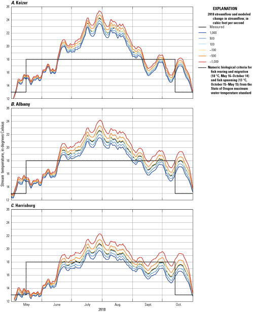
Predicted stream temperature from regression models using 2018 air temperatures and variations from measured 2018 streamflow conditions at (A) Keizer, (B) Albany, and (C) Harrisburg along the Willamette River, northwestern Oregon. The dashed black line indicates the numeric biological criteria for fish rearing and migration (18 °C, May 16–October 14) and fish spawning (13 °C, October 15–May 15) from the State of Oregon maximum water-temperature standard.
Table 7.
Predicted annual maximum 7-day average of the daily maximum (7dADMax) and monthly means of 7dADMax water temperature for 2018 at Keizer, Albany, and Harrisburg, Willamette River, northwestern Oregon.[Predictions use the regressions models for each site, applying measured air temperatures from 2018 and variations from the measured 2018 streamflow conditions. Temperatures are in degrees Celsius. ft3/s, cubic feet per second]
Flow modifications of discrete magnitudes influence stream temperature in proportion to the percent change in resulting flow that the modification represents. As a result, discrete flow modifications, such as might be implemented at a particular dam, will produce a greater effect at upstream locations where the change in flow represents a greater percent of total flows. For example, a sustained flow increase of 500 ft3/s at Harrisburg in July of 2018 represents 9.6 percent of the resulting streamflow and is predicted to produce an average monthly decrease in the 7dADMax temperature of 0.5 °C (table 6). Farther downstream at Keizer, however, 500 ft3/s is only 6.6 percent of the resulting July flow and is estimated to decrease the monthly mean 7dADMax temperature in July 2018 by only 0.3 °C. Similarly, because a set increase in streamflow represents a smaller percentage of the final flow when compared to a set decrease in streamflow, the temperature effect of decreasing streamflow is magnified compared to the effect of a similar streamflow increase. For example, a sustained decrease in flow of 500 ft3/s at Harrisburg represents 11.8 percent of the resulting average monthly flow and produces a predicted temperature increase of 0.6 °C, as compared to the 0.5 °C decrease predicted for a similar flow increase. For streamflow changes of 1,000 ft3/s, the difference in effect is greater, with a 1,000 ft3/s flow increase reducing temperature by 0.9 °C while a similar decrease in streamflow increases stream temperatures by 1.4 °C for July at Harrisburg (table 6).
Discussion
Regression-based models of varying form and input requirements have shown good success in predicting stream temperature across a broad range of landscapes and timescales (Johnson, 1971; Mohseni and others, 1998; Donato, 2002; Isaak and others, 2017). For example, using a nonlinear regression model relating weekly air temperature to weekly stream temperature, Mohseni and others (1998) reported an RMSE of 1.64 ±0.46 °C using data from 584 USGS gaging stations. Donato (2002) used seasonal temperature fluctuations, site elevation, total drainage area, average subbasin slope, and the deviation of the daily average air temperature from a 30-year normal average air temperature to calculate daily average stream temperature in August and September with a reported RMSE range of 1.3–2.1 °C. More recently, research has been successful in applying a range of hydrologic and geomorphic covariates to develop spatial-stream-network models of mean August stream temperature at 1-kilometer intervals, with a reported RMSE of 1.1 °C (Isaak and others, 2017).
The seasonally based, piecewise approach to multiple linear regression with smoothed seasonal transition multipliers, as applied in this study, has several advantages. First, with only two covariates (streamflow and air temperature), the models are relatively simple to construct and implement. Second, by applying a seasonal, smoothed piece-wise approach, the models can produce an annual time series of estimated temperature that accounts for seasonal variability in the relations among water temperature, air temperature, and streamflow. Seasonal model fits are good in winter, spring, and summer and worse in early and late autumn (fig. 11; tables 1.1–1.12), probably because of variation in the timing and magnitude of winter storms in the Willamette River basin and the associated end of the summer low-flow season. The resulting smoothed annual models produced annual MAE values of 0.4–0.9 °C for the 7dADMean and 0.5–1.0 °C for the 7dADMax (table 2), a range of uncertainty within the 1 °C maximum MAE benchmark typically used to characterize acceptable results from a mechanistic water-temperature model. The use of a daily, week-averaged time scale by these regression models coincides with the regulatory criteria applicable to stream temperature in Oregon. The weekly time scale also helps to prevent any substantial influence of lag times or autocorrelation in the shorter time-scale (diurnal or shorter) responses of stream temperature to covariate variation (see Caissie, 2006; Letcher and others, 2016).
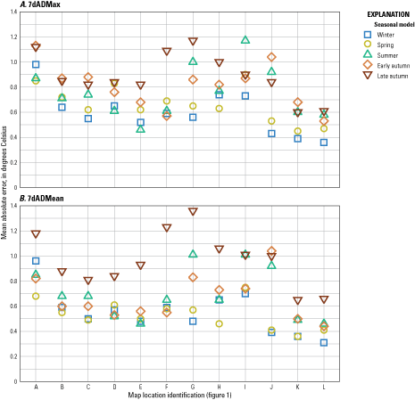
Graphs showing the mean absolute error (MAE) by seasonal model for the (A) 7-day average of the daily maximum (7dADMax) and (B) 7-day average of the daily mean (7dADMean). Letter designations correspond to map locations shown in figure 1.
The accuracy of the regression models demonstrates that air temperature and streamflow are reasonable proxies for the processes influencing stream temperature in the Willamette River and its major tributaries, but that the strength and relative importance of processes controlling stream temperature vary seasonally and spatially within the river network. The association between air temperature and stream temperature is strongest during the warming and cooling seasons of spring and autumn, while at the low and high ends of the air temperature range, the relation between air temperature and stream temperature begins to curve and “flatten” out (figs. 3–4). The “flattening out” at lower air temperatures has been attributed in other studies to the influence of groundwater, which has also been found to reduce the slope of the air temperature to stream temperature relation (Mohseni and others, 1998; Caissie, 2006). This theory is supported by comparing the slope of the relation between air temperature and stream temperature on groundwater- versus surface-water-dominated streams. For example, the relation between air temperature and stream temperature on the McKenzie River, which is dominated by groundwater inputs (Conlon and others, 2005; Tague and others, 2007), has a much lower slope than the same relation at non-groundwater dominated sites like Goshen on the Coast Fork Willamette River (figs. 3–4). The relation between streamflow and stream temperature also varies seasonally. Stream temperatures are closely coupled to streamflow in the spring through early autumn but relatively independent in late autumn and winter, when streamflows are high (figs. 5–6). Consequently, flow modifications during this cold winter period are unlikely to have a substantial influence on stream temperature. Additionally, the influence of flow augmentation on stream temperature in summer and early autumn is greater in most years than in spring and early summer. In spring and early summer, while insolation (the amount of solar radiation reaching a given area) is highest, spring snowmelt and runoff are also typically high. In contrast, baseflow is typically low in summer and early autumn. Flow modifications can thus represent a greater percentage of total flow and have a larger influence on stream temperature.
In the reaches immediately below USACE dams, stream temperature is strongly controlled by the temperature of dam releases, which in turn is determined by the timing and depth of thermal stratification in conjunction with lake level, dam-outlet depths, and dam operations (Rounds, 2007; Rounds, 2010). Water-quality studies conducted during the 1970s noted that cold water released from Lookout Point Lake on the Middle Fork Willamette River influenced stream temperatures as far downstream as RM 120 (upstream of Albany), and particularly upstream of RM 172 between Harrisburg and the confluence of the Willamette and McKenzie Rivers (Hines and others, 1977). More recent modeling work showed that the effect of dam releases on downstream water temperature can be as much as 4–5 °C in the Willamette River upstream of the McKenzie River confluence at RM 174.9 but less than 1°C, under typical conditions, downstream of the Santiam River confluence at RM 108.5 (Rounds, 2010). This modeling also showed that dam releases cause disruptions in the natural seasonal warming and cooling patterns of downstream river reaches, with slower warming and later cooling than under a no-dam scenario (Rounds, 2010), a pattern that has been observed in the data from streamgages across the United States (Mohseni and others, 1998, 1999). Study locations that were close to dams (for example, the Middle Fork Willamette River at Jasper, which is 10.3 RM downstream of Fall Creek Dam and 8.7 RM downstream from Dexter Dam) showed strong seasonal hysteresis (figs. 3–4), which was probably indicative of the lag in warming and cooling observed by previous research. However, the delayed warming effect of dams during spring may be confounded by the effect of spring snowmelt, which depresses the rate of spring warming relative to autumn cooling (Webb and Nobilis, 1999; Lisi and others, 2015).
The dependency of stream temperature on streamflow and air temperature assumes that these metrics are reliable proxies for the heat flux processes influencing stream temperature at a given location. Thus, the regression methods applied in this study could not generally be used to model stream temperature with acceptable accuracy at locations where dam operations may unpredictably change the temperature of release from season to season or year to year. The distance (or travel time) from a dam to a point at which stream temperatures can be reasonably approximated by air temperature and streamflow will vary seasonally and according to local conditions. Variability in model fit at locations relatively near dams can thus provide insight into the conditions and heat flux processes at these sites. For example, given their proximity to upstream dams (fig. 1), regression models for the McKenzie River at Vida (approximately 16 mi downstream of Cougar Dam and 10.5 mi downstream of Blue River Dam) would be expected to be relatively poor. However, with a relatively small MAE of 0.4 °C for the 7dADMean, the McKenzie River at Vida has one of the best model fits in the basin (table 2). This good model performance, despite being closer to some upstream dams than streamgages on other rivers with poor fits, is explained by the facts that (1) the USACE dam releases contribute a small percentage of the total flow in the McKenzie River and (2) the upper McKenzie River is highly influenced by large and relatively stable groundwater inputs, which causes more stable temperature patterns that are easier to reproduce from year to year. Elsewhere, the relatively good model fit statistics for models applied at locations near upstream dams (such as the Middle Fork Willamette River at Jasper, 8.7 mi from Dexter Dam and 10.3 mi from Fall Creek Dam) suggest that the influence of upstream dam releases diminishes relatively rapidly with time and downstream distance at some locations or that they are very consistent from year to year. This implies that heat exchange of these rivers with the environment is potentially rapid and that the accumulated environmental heat fluxes over several days can replace much of the heat content of the water released at the upstream dams. The rapid heat exchange in these reaches may in part reflect channel morphology and features, such as numerous shallow riffles and a relatively large width-to-depth ratio, that allow rapid adjustment to environmental heat fluxes.
In reaches sufficiently downstream that the influence of dam release temperatures is minimal, model results indicate that summer stream temperatures vary more at downstream locations than at upstream locations from a very hot and very dry year to a cool and very wet year (fig. 9). This pattern in the results suggests that low streamflow and high air temperatures may disproportionately affect downstream reaches of the Willamette River, such as Keizer, as compared to more-upstream locations such as Harrisburg. Conversely, the thermal consequences of a discrete change in streamflow (for example, ±500 ft3/s) are greater at more-upstream locations where that change likely represents a greater percentage of total streamflow and thus has a greater relative effect on travel time and thermal mass than it would at more-downstream locations where additional tributary inflows would dilute the effect (table 6). Although the warming effect of a constant flow decrease at Harrisburg is predicted to be greater than at Keizer, modeling results from 2018 suggest that the magnitude of the difference can vary seasonally. As modeled, the influence of a flow increase or decrease on stream temperature would have been relatively small and hard to detect until mid-June, when a decrease in flow coincided with a large increase in air temperature. After mid-June of 2018, opportunities to affect stream temperature through flow management increased. An examination of the seasonal model coefficients for air temperature and streamflow for the Harrisburg and Keizer sites (tables 1.3, 1.5) shows that the influence of air temperature on the 7dADMean stream temperature decreases at Harrisburg from spring to early autumn (coefficients decreasing from 0.51 to 0.37) but stays relatively constant at Keizer (coefficients between 0.49 and 0.51). In contrast, the effect of streamflow at Keizer is stronger in spring and decreases through summer and early autumn (coefficients decreasing from 49,852 to 28,876), whereas the streamflow effect at Harrisburg increases slightly from spring to summer and then decreases somewhat in early autumn (coefficients of 21,272, 22,176, and 14,082). This implies that climate conditions may be more important in controlling stream temperature at the more-downstream sites, and streamflow management to modify water temperature may be more effective at the more-upstream sites through summer and early autumn, depending on the magnitude of streamflow.
Finally, model analyses of the historical range of air temperature and streamflow conditions indicate that, under current geomorphic conditions and flow-management strategies, the Willamette River as far upstream as Harrisburg likely will continue to exceed the State of Oregon maximum water-temperature criterion of 18 °C from late spring to early autumn for sustained periods and that flow management, while effective, likely cannot prevent such exceedances. Cooler conditions below 18 °C were predicted at Harrisburg only in cool (below normal air temperature) and very wet (much-above normal streamflow) years. Temperatures exceeded 18 °C for much of the summer at more-downstream sites such as Albany and Keizer even in cool and very wet years. For much-above normal air-temperature conditions, model results suggest that the mean July 7dADMax at Keizer could range from 21.2 to 23.7 °C, depending on streamflow, while average July 7dADMax at Harrisburg could be as high as 18.7–20.8 °C (table 3). As modeled for 2018, sustained flow augmentation of 1,000 ft3/s decreased the mean July 7dADMax at Keizer from 21.9 to 21.3 °C (table 7). If summertime air temperature continues to warm in a changing climate, such changes will exacerbate warm water-temperature conditions in the Willamette River stream network (Chang and others, 2018).
Model Limitations
The models developed in this study provide a simple and relatively accurate means of estimating stream temperature at key locations along the main channel of the Willamette River and its major tributaries; however, the accuracy of the modeled stream temperatures is subject to several limitations. First, because the models are statistical rather than mechanistic, they are best used within the range of air temperature and streamflow conditions use to construct the models; extrapolation beyond that range will introduce an increasing amount of uncertainty in the predictions. Data beyond the range of that included in the models cannot be assumed to follow the same pattern. In particular, confidence in stream temperature estimates from low streamflow conditions is limited by the relative paucity of low-streamflow inputs to the models (figs. 5–6); as a result, analyses of the effects of additional withdrawals or of streamflow conditions below the typical range used for model construction may represent extrapolations and should be interpreted with care. For example, it is important to remember that low-flow summer streamflows in the Willamette River are roughly twice as high as those prior to completion of several large dams in the early 1950s (Rounds, 2010) and that extrapolation to such pre-dam streamflow conditions is not recommended with these regression models. As an aid to determining the conditions under which the regression models are valid at each location, figs. 1.1–1.2 depict the seasonal range of air temperature and streamflow data included in the statistical model for each location. Stream temperatures calculated using input values that plot outside the range of measured data are subject to greater uncertainty than those that plot within it; for example, stream temperature predictions calculated using streamflows below about 3,700 ft3/s at Albany in the summer and early autumn are subject to greater uncertainty than stream temperature predictions calculated using streamflows of about 6,000 ft3/s.
Second, because air temperature and streamflow are proxies for the environmental heat fluxes and other processes influencing stream temperature, any substantial changes to the river environment that may influence flow paths, residence time, river width or depth, and (or) riparian shading likely will alter the accuracy and suitability of the models developed in this study and require the development of updated models. This statement has two implications: first, although the models developed in this study are relatively accurate for describing temperature relations occurring in the river system as it exists, such models cannot be applied with confidence to estimate stream temperatures under substantially altered future conditions, when the relation between various heat fluxes might be altered enough that the model coefficients developed here are no longer the best description of the relations between air temperature, streamflow, and stream temperature. Similarly, the regression models cannot be used to “hindcast” historical conditions in the river when flow regimes, channel morphology, riparian vegetation and sediment supply were significantly different than they are today (Sedell and Froggatt, 1984; Wallick and others, 2013).
Although the regression models provide an effective means to investigate the sensitivity of stream temperature to flow management, the simple model inputs (air temperature and streamflow) cannot account for the direct influence of dam release temperatures, the competing effects of adjustments in flow releases from multiple upstream dam locations, and the heat-content alterations that a water parcel undergoes while in transit to a particular location; therefore, these models cannot effectively predict all of the intricacies of flow management strategies involving multiple upstream reservoirs. Additionally, the greater error in regression models at sites closer to upstream dams (for example, the North Santiam River at/near Mehama or the Santiam River near Jefferson) provides evidence that upstream dam operations influence stream temperature in ways not captured by these simple models. As a result, while the regression models can be reliably used to estimate stream temperature response to an additional 100 or 500 ft3/s of streamflow in the Willamette River at Keizer, they cannot be used to determine the implications of, for example, garnering that additional streamflow from releases from Detroit Lake in the North Santiam River basin versus Lookout Point Lake in the Middle Fork Willamette River basin or the effect of releasing water over the spillway versus through the power penstocks of Detroit Dam. For these types of determinations, a mechanistic model such as CE-QUAL-W2 (Wells, 2019) can better account for the influence of variable boundary conditions, the evolution of stream heat budgets with downstream travel time, the effects of dam operations, and other processes influencing heat fluxes on stream temperature (for example, see Rounds, 2010; Buccola and others, 2013; Buccola, 2017).
While the regression models developed in this study are based on weekly averages and the State of Oregon maximum water-temperature standard is based on the 7dADMax, a weekly timescale obscures diel patterns and smooths anomalous daily peaks in temperature that likely have ecological importance. The regression models developed in this study are simple tools that are valuable for garnering insights into the potential effects of flow-management strategies or changes in climate, and their simplicity allows for computationally fast and efficient analysis of long datasets or coupling to other models or decision-support systems, but the models also are limited by that simplicity. With respect to spatial scales, the regression models estimate stream temperature at the measurement location of the streamgage, and the predicted temperature therefore can be assumed to represent the near-isothermal and mixed conditions in the main channel. Depending on the geomorphology of individual reaches, however, some significant thermal heterogeneity (and diversity of fish habitat) may occur in off-channel environments or in tributary plumes that is not captured by these models. Furthermore, while the assumption that the temperature data collected by USGS streamgages represent well-mixed, isothermal conditions in the main channel is reasonable, there may be variability in temperature conditions in the main channel not accounted for by these models or the data records used to build them. Investigating cross-sectional variability in thermal conditions in the Willamette River is beyond the scope of this study but would be valuable future work.
Finally, while the accuracy of the regression equations developed in this report varies by location, the regression equations developed for Willamette Falls are unique and should be applied with greater caution. Because the original data used to build the regression equations for that site are themselves derived from a regression with stream temperature measurements at Newberg and an incomplete daily temperature dataset at Willamette Falls, the goodness-of-fit statistics presented in tables 2 and 1.1 do not reflect a comparison with actual measurements. Additionally, while correlation between the data provided by ODFW and the limited USGS data available from Willamette Falls is good and appears to be unbiased, the ODFW dataset may not meet USGS data-quality standards. Thus, while the regression relations developed for Willamette Falls can provide useful information, uncertainty in the relation at Willamette Falls is relatively high, and interpretations made from temperature estimates for that site should be made with care.
Summary and Conclusions
This report documents the development of regression relations used to estimate the 7-day moving average of the daily mean (7dADMean) and the 7-day moving average of the daily maximum (7dADMax) stream temperature at 12 locations on the Willamette River and major tributaries downstream of U.S. Army Corps of Engineers dams. Regression models were developed as tools to investigate the thermal regimes of the river network and its sensitivity to weather and climate variations and to better understand the potential for flow management to influence stream temperature. Using publicly available records of air temperature, streamflow, and stream temperature, a smoothed and piecewise multiple linear regression approach was used to build stream temperature models with annual MAE ranging from 0.4 to 0.9 °C (7dADMean) and 0.5 to 1.0 °C (7dADMax) and RMSE ranging from 0.6 to 1.1 °C (7dADMean) and 0.6 to 1.2 °C (7dADMax). Goodness-of-fit statistics for the models show that air temperature and streamflow are reasonable proxies for the processes influencing stream temperature in the Willamette River stream network except at locations relatively close to upstream dams where the temperature of dam releases is important. These analyses suggest that environmental heat fluxes across the river surface in the Willamette River system during spring through autumn are large compared to the heat content of the river, such that stream temperature in the Willamette River and the lower reaches of its major tributaries is primarily controlled by those environmental heat fluxes, and less so by the temperature of upstream dam releases.
Modeled responses to flow management strategies in the Willamette River system suggest that the sensitivity of water temperature in the Willamette River to flow management varies based on location. As modeled for 2018 (a very hot year with average to below-average streamflow), changes in streamflow ranging from ±100 to ±1,000 ft3/s produced mean monthly temperature changes from 0.0 to 1.4 °C, depending on the time of year. Large decreases in streamflow produced larger changes in temperature than did similar levels of flow augmentation. Although modeling of pre-dam conditions is beyond the capability of these regression models because such low streamflows would be well outside the range of calibrated conditions, preferentially larger increases in stream temperature associated with decreases in streamflow imply that adjusting to a more “natural” (non-augmented) flow regime during summer would cause substantial warming in the river system. However, model results suggest that flow augmentation can effectively contract the duration of summer temperatures exceeding 18 °C, particularly at more-upstream sites such as Harrisburg where temperatures tend to be lower than at more-downstream sites.
The regression models developed in this study indicate that, because of the greater influence of changes in streamflow at relatively low-flow conditions, the potential for flow management to influence stream temperature is (1) greater at upstream locations as compared to downstream locations and (2) likely to be more effective in summer and autumn when streamflow is low, as opposed to during spring when streamflow tends to be higher. Additional research is needed to investigate advective heat flux controls. The dominance of source-related advective heat flux on stream temperature in winter and spring suggests that, as climate warms and winter precipitation shifts to rain versus snow, spring warming may show an enhanced response to climate change. Furthermore, this effect may be compounded by a decrease in the spring snowmelt signature.
Although the models developed in this study rely on empirical relations to estimate stream temperature, a better understanding of the relations among water temperature, air temperature, and streamflow provides valuable insights into the dominant controls on stream temperature in the Willamette River, the seasonal variation of those controls, and the sensitivity of stream temperature in the Willamette River system to flow management. The simplicity of the statistical modeling approach and the requirement of only two readily available model inputs (air temperature and streamflow) allows for rapid model development and deployment, and therefore can be easily applied to evaluate a wide range of management questions. These results and insights are valuable for water-resource managers, regulators, and scientists who may need to develop strategies to evaluate and optimize flow management strategies to improve the health, survival, and habitats of threatened fish populations.
References Cited
Brown, G.W., 1969, Predicting temperatures of small streams: Water Resources Research, v. 5, no. 1, p. 68–75, https://doi.org/10.1029/WR005i001p00068.
Buccola, N.L., Stonewall, A.J., Sullivan, A.B., Kim, Y., and Rounds, S.A., 2013, Development of CE-QUAL-W2 models for the Middle Fork Willamette and South Santiam Rivers, Oregon: U.S. Geological Survey Open File Report 2103–1186, 55 p., https://doi.org/10.3133/ofr20131186.
Buccola, N.L., 2017, Water temperature effects from simulated changes to dam operations and structures in the Middle and South Santiam Rivers, Oregon: U.S. Geological Survey Open-File Report 2017–1063, 19 p., https://doi.org/10.3133/ofr20171063.
Bladon, K.D., Segura, C., Cook, N.A., Bywater-Reyes, S., and Reiter, M., 2018, A multicatchment analysis of headwater and downstream temperature effects from contemporary forest harvesting: Hydrological Processes, v. 32, no. 2, p. 293–304. https://doi.org/10.1002/hyp.11415.
Caissie, D., 2006, The thermal regime of rivers—A review: Freshwater Biology, v. 51, no. 8, p. 1389–1406, https://doi.org/10.1111/j.1365-2427.2006.01597.x.
Chang, H., Watson, E., and Strecker, A., 2018, Climate change and stream temperature in the Willamette River Basin: implications for stream habitat, chap. 8 of Bridging science and policy implication for managing climate extremes, Jung, H., and Wang, B., eds.: World Scientific, World Scientific Series on Asia-Pacific Weather and Climate, v. 10, 232 p., https://doi.org/10.1142/9789813235663_0008.
Conlon, T.D., Wozniak, K.C., Woodcock, D., Herrera, N.B., Fisher, B.J., Morgan, D.S., Lee, K.K., and Hinkle, S.R., 2005, Ground-water hydrology of the Willamette Basin, Oregon: U.S. Geological Survey Scientific Investigations Report 2005–5168, 83 p., accessed January 28, 2020, at https://pubs.usgs.gov/sir/2005/5168/.
Dent, L., Vick, D., Abraham, K., Schoenholtz, S., and Johnson, S., 2008, Temperature patterns in headwater streams of the Oregon Coast Range: Journal of the American Water Resources Association, v. 44, no. 4, p. 803–813, https://doi.org/10.1111/j.1752-1688.2008.00204.x.
Donato, M.M., 2002, A statistical model for estimating stream temperatures in the Salmon and Clearwater River Basins, central Idaho: U.S. Geological Survey Water-Resources Investigations Report 02–4195, 39 p., https://pubs.usgs.gov/wri/2002/4195/report.pdf.
Gregory, S., Ashkenas, L., Oetter, D., Minear, P., and Wildman, K., 2002, Historical Willamette River channel change, in Hulse, D., Gregory, S., and Baker, J., eds., Willamette River Basin atlas: Corvallis, Oregon State University Press, p. 18–24, accessed July 7, 2020, at http://www.fsl.orst.edu/pnwerc/wrb/Atlas_web_compressed/3.Water_Resources/3c.historic_chl_web.pdf.
Hansen, A.C., Kock, T.J., and Hansen, G.S., 2017, Synthesis of downstream fish passage information at projects owned by the U.S. Army Corps of Engineers in the Willamette River Basin, Oregon: U.S. Geological Survey Open File Report 2017–1101, 118 p., https://doi.org/10.3133/ofr20171101.
Hines, W.G., McKenzie, S.W., Rickert, D.A., and Rinella, F.A., 1977, Dissolved-oxygen regimen of the Willamette River, Oregon, under conditions of basinwide secondary treatment—River-quality assessment of the Willamette River Basin, Oregon: US Geological Survey Circular 715–I, 66 p., accessed October 23, 2019, at https://pubs.er.usgs.gov/publication/cir715I.
Ingebritsen, S.E., Mariner, R.H., and Sherrod, D.R., 1994, Hydrothermal systems of the Cascade Range, north-central Oregon: U.S. Geological Survey Professional Paper 1044-L, 85 p., https://pubs.usgs.gov/pp/1044l/report.pdf.
Isaak, D.J., Wenger, S.J., Peterson, E.E., Ver Hoef, J.M., Nagel, D.E., Luce, C.H., Hostetler, S.W., Dunham, J.B., Roper, B.B., Wollrab, S.P., Chandler, G.L., Horan, D.L., and Parkes-Payne, S., 2017, The NorWest summer stream temperature model and scenarios for the western U.S.—A crowd-sourced database and new geospatial tools foster a user community and predict broad climate warming of rivers and streams: Water Resources Research, v. 53, no. 11, p. 9181–9205, https://doi.org/10.1002/2017WR020969.
Jefferson, A., Grant, G., and Rose, T., 2006, Influence of volcanic history on groundwater patterns on the west slope of the Oregon High Cascades: Water Resources Research, v. 42, p. 1–15, https://doi.org/10.1029/2005WR004812.
Johnson, F.A., 1971, Stream temperatures in an alpine area: Journal of Hydrology, v. 14, nos. 3–4, p. 322–336, https://doi.org/10.1016/0022-1694(71)90042-4.
Letcher, B.H., Hocking, D.J., O’Neil, K., Whiteley, A.R., Nislow, K.H., and O’Donnell, M.J., 2016, A hierarchical model of daily stream temperature using air-water temperature synchronization, autocorrelation, and time lags: PeerJ, v. 4, p. e1727, https://doi.org/10.7717/peerj.1727.
Lisi, P.J., Schindler, D.E., Cline, T.J., Scheuerell, M.D., and Walsh, P.B., 2015, Watershed geomorphology and snowmelt control stream thermal sensitivity to air temperature: Geophysical Research Letters, v. 42, no. 9, p. 3380–3388, https://doi.org/10.1002/2015GL064083.
McCulloch, D.A., 1999, A review and synthesis of effects of alterations to the water temperature regime of freshwater life stages of salmonids, with special reference to Chinook salmon: EPA-910-R-99-010, 279 p., accessed October 23, 2019, at https://www.critfc.org/wp-content/uploads/2012/11/EPAreport_2.pdf.
Mohseni, O., Erickson, T.R., and Stefan, H.G., 1999, Sensitivity of stream temperatures in the United States to air temperatures projected under a global warming scenario: Water Resources Research, v. 35, no. 12, p. 3723–3733, https://doi.org/10.1029/1999WR900193.
Mohseni, O., Stefan, H.G., and Erickson, T.R., 1998, A nonlinear regression model for weekly stream temperatures: Water Resources Research, v. 34, no. 10, p. 2685–2692, https://doi.org/10.1029/98WR01877.
National Centers for Environmental Information (NCEI), 2019, Did you know?: National Oceanic and Atmospheric Administration web page, accessed October, 20, 2019, at https://www.ncdc.noaa.gov/monitoring-references/dyk/ranking-definition.
National Centers for Environmental Information (NCEI), 2020, Climate at a glance—Divisional time series: National Oceanic and Atmospheric Administration web site, accessed April 17, 2020, at https://www.ncdc.noaa.gov/cag/.
National Marine Fisheries Service, 1999, Updated review of the status of the upper Willamette River and middle Columbia River ESUs of steelhead (Oncorhynchus mykiss): National Marine Fisheries Service West Coast Steelhead Biological Review Team, https://repository.library.noaa.gov/view/noaa/21171.
National Marine Fisheries Service, 2008, Willamette Basin Biological Opinion—Endangered Species Act Section 7(a)(2) Consultation: National Marine Fisheries Service, NOAA Fisheries Log Number F/NWR/2000/02117 [variously paged], accessed October 23, 2019, at https://www.fisheries.noaa.gov/resource/document/consultation-willamette-river-basin-flood-control-project.
Neumann, D.W., Rajagopalan, B., and Zagona, E.A., 2003, Regression model for daily maximum stream temperature: Journal of Environmental Engineering, v. 129, no. 7, p. 667–674, https://doi.org/10.1061/(ASCE)0733-9372(2003)129:7(667).
Oregon Department of Environmental Quality, 2003, Figure 340A—Fish use designations Willamette Basin, Oregon: Oregon Department of Environmental Quality, accessed October 23, 2019, at https://www.oregon.gov/deq/FilterRulemakingDocs/figure340a.pdf.
Oregon Department of Environmental Quality, 2005, Draft revised Figure 340B—Salmon and steelhead spawning use designations, Willamette Basin, Oregon: Oregon Department of Environmental Quality, accessed October 23, 2019, at https://www.oregon.gov/deq/FilterRulemakingDocs/figure340b.pdf.
Oregon Department of Environmental Quality, 2020, Water quality standards—Beneficial uses, policies, and criteria for Oregon—Temperature: Oregon Administrative Rule 340-041-0028(4), Oregon Department of Environmental Quality, accessed January 30, 2020, at https://secure.sos.state.or.us/oard/viewSingleRule.action?ruleVrsnRsn=244176.
PRISM Climate Group, Oregon State University, 2020, PRISM climate data: Corvallis, Prism Climate Group, Oregon State University website, accessed April 28, 2020, at http://www.prism.oregonstate.edu.
Poole, G.C., and Berman, C.H., 2001, An ecological perspective on in-stream temperature—Natural heat dynamics and mechanisms of human-caused thermal degradation: Environmental Management, v. 27, no. 6, p. 787–802, https://doi.org/10.1007/s002670010188.
R Core Team, 2018, R—A language and environment for statistical computing: Vienna, Austria, R Foundation for Statistical Computing, version 3.5.2 “Eggshell Igloo,” accessed January 1, 2019, at https://www.R-project.org/.
Risley, J.C., Constantz, J.A., Essaid, H.I., and Rounds, S.A., 2010, Effects of upstream dams versus groundwater pumping on stream temperature under varying climate conditions: Water Resources Research, v. 46, no. 6, W06517, https://doi.org/10.1029/2009WR008587.
Rounds, S.A., 2007, Temperature effects of point sources, riparian shading, and dam operations on the Willamette River, Oregon: U.S. Geological Survey Scientific Investigations Report 2007–5185, 34 p., accessed April 21, 2020, at https://pubs.usgs.gov/sir/2007/5185/.
Rounds, S.A., 2010, Thermal effects of dams in the Willamette River basin, Oregon: U.S. Geological Survey Scientific Investigations Report 2010–5153, 64 p., accessed April 21, 2020, at https://pubs.usgs.gov/sir/2010/5153/.
Sedell, J.R., and Froggatt, J.L., 1984, Importance of streamside forests to large rivers—The isolation of the Willamette River, Oregon, U.S.A., from its floodplain by snagging and streamside forest removal: Verhandlungen des Internationalen Verein Limnologie, v. 22, p. 1828–1834, accessed January 8, 2021, at https://andrewsforest.oregonstate.edu/sites/default/files/lter/pubs/pdf/pub1990.pdf.
Stratton Garvin, L., 2022, Stream temperature predictions for the Willamette River Basin, northwestern Oregon estimated from regression equations (1954–2018): U.S. Geological Survey data release, https://doi.org/10.5066/P9PALKQZ.
Tague, C., and Grant, G., 2004, A geological framework for interpreting the low-flow regimes of Cascade streams, Willamette River Basin, Oregon: Water Resources Research, v. 40, no. 4, W04303, https://doi.org/10.1029/2003WR002629.
Tague, C., Farrell, M., Grant, G., Lewis, S., and Rey, S., 2007, Hydrogeologic controls on summer stream temperatures in the McKenzie River basin, Oregon: Hydrological Processes, v. 21, no. 24, p. 3288–3300, https://doi.org/10.1002/hyp.6538.
U.S. Geological Survey, 2019, National Water Information System: U.S. Geological Survey web page, accessed October 29, 2019, at https://dx.doi.org/10.5066/F7P55KJN.
Wallick, J.R., Jones, K.L., O’Connor, J.E., Keith, M.K., Hulse, D., and Gregory, S.V., 2013, Geomorphic and vegetation processes of the Willamette River floodplain, Oregon—Current understanding and unanswered questions: U.S. Geological Survey Open-File Report 2013–1246, 70 p., https://doi.org/10.3133/ofr20131246.
Webb, B.W., and Nobilis, F., 1999, Long-term perspective on the nature of the air-water temperature relationship—A case study: Hydrological Processes, v. 11, no. 2, p. 137–147, https://doi.org/10.1002/(SICI)1099-1085(199702)11:2<137::AID-HYP405>3.0.CO;2-2.
Wilkinson, G.N., and Rogers, C.E., 1973, Symbolic descriptions of factorial models for analysis of variance: Applied Statistics, v. 22, no. 3, p. 392–399, https://doi.org/10.2307/2346786.
Appendix 1. Model Evaluation and Applications
Table 1.1.
Regression coefficients and goodness-of-fit statistics for the water-temperature model for the study site (Location A) at the Willamette River at River Mile 26.6, Willamette Falls, northwestern Oregon.[Location A is shown in figure 1. All temperatures in the models were in degrees Celsius and all streamflows were in cubic feet per second. Abbreviations: ME, mean error; MAE, mean absolute error; RMSE, root mean square error; °C, degrees Celsius; 7dADMean, 7-day average of the daily mean; 7dADMax, 7-day average of the daily maximum]
Table 1.2.
Regression coefficients and goodness-of-fit statistics for the water-temperature model for the study site (Location B) at the Willamette River at Newberg (USGS 14197900), northwestern Oregon.[Location B is shown in figure 1. All temperatures in the models were in degrees Celsius and all streamflows were in cubic feet per second. Abbreviations: ME, mean error; MAE, mean absolute error; RMSE, root mean square error; °C, degrees Celsius; 7dADMean, 7-day average of the daily mean; 7dADMax, 7-day average of the daily maximum]
Table 1.3.
Regression coefficients and goodness-of-fit statistics for the water-temperature model for the study site (Location C) at the Willamette River at Keizer (USGS 14192015), northwestern Oregon.[Location C is shown in figure 1. All temperatures in the models were in degrees Celsius and all streamflows were in cubic feet per second. Abbreviations: ME, mean error; MAE, mean absolute error; RMSE, root mean square error; °C, degrees Celsius; 7dADMean, 7-day average of the daily mean; 7dADMax, 7-day average of the daily maximum]
Table 1.4.
Regression coefficients and goodness-of-fit statistics for the water-temperature model for the study site (Location D) at the Willamette River at Albany (USGS 14174000), northwestern Oregon.[Location D is shown in figure 1. All temperatures in the models were in degrees Celsius and all streamflows were in cubic feet per second. Abbreviations: ME, mean error; MAE, mean absolute error; RMSE, root mean square error; °C, degrees Celsius; 7dADMean, 7-day average of the daily mean; 7dADMax, 7-day average of the daily maximum]
Table 1.5.
Regression coefficients and goodness-of-fit statistics for the water-temperature model for the study site (Location E) at the Willamette River at Harrisburg (USGS 14166000), northwestern Oregon.[Location E is shown in figure 1. All temperatures in the models were in degrees Celsius and all streamflows were in cubic feet per second. Abbreviations: ME, mean error; MAE, mean absolute error; RMSE, root mean square error; °C, degrees Celsius; 7dADMean, 7-day average of the daily mean; 7dADMax, 7-day average of the daily maximum]
Table 1.6.
Regression coefficients and goodness-of-fit statistics for the water-temperature model for the study site (Location F) at the Willamette River at Owosso Bridge at Eugene (USGS 14158100), northwestern Oregon.[Location F is shown in figure 1. All temperatures in the models were in degrees Celsius and all streamflows were in cubic feet per second. Abbreviations: ME, mean error; MAE, mean absolute error; RMSE, root mean square error; °C, degrees Celsius; 7dADMean, 7-day average of the daily mean; 7dADMax, 7-day average of the daily maximum]
Table 1.7.
Regression coefficients and goodness-of-fit statistics for the water-temperature model for the study site (Location G) at the Middle Fork Willamette River at Jasper (USGS 14152000), northwestern Oregon.[Location G is shown in figure 1. All temperatures in the models were in degrees Celsius and all streamflows were in cubic feet per second. Abbreviations: ME, mean error; MAE, mean absolute error; RMSE, root mean square error; °C, degrees Celsius; 7dADMean, 7-day average of the daily mean; 7dADMax, 7-day average of the daily maximum]
Table 1.8.
Regression coefficients and goodness-of-fit statistics for the water-temperature model for the study site (Location H) at the Coast Fork Willamette River near Goshen (USGS 14157500), northwestern Oregon.[Location H is shown in figure 1. All temperatures in the models were in degrees Celsius and all streamflows were in cubic feet per second. Abbreviations: ME, mean error; MAE, mean absolute error; RMSE, root mean square error; °C, degrees Celsius; 7dADMean, 7-day average of the daily mean; 7dADMax, 7-day average of the daily maximum]
Table 1.9.
Regression coefficients and goodness-of-fit statistics for the water-temperature model for the study site (Location I) at the Santiam River near Jefferson (USGS 14189050), northwestern Oregon.[Location I is shown in figure 1. All temperatures in the models were in degrees Celsius and all streamflows were in cubic feet per second. Abbreviations: ME, mean error; MAE, mean absolute error; RMSE, root mean square error; °C, degrees Celsius; 7dADMean, 7-day average of the daily mean; 7dADMax, 7-day average of the daily maximum]
Table 1.10.
Regression coefficients and goodness-of-fit statistics for the water-temperature model for the study site (Location J) at the North Santiam River at/near Mehama (USGS 14183000/14183010), northwestern Oregon.[Location J is shown in figure 1. All temperatures in the models were in degrees Celsius and all streamflows were in cubic feet per second. Abbreviations: ME, mean error; MAE, mean absolute error; RMSE, root mean square error; °C, degrees Celsius; 7dADMean, 7-day average of the daily mean; 7dADMax, 7-day average of the daily maximum]
Table 1.11.
Regression coefficients and goodness-of-fit statistics for the water-temperature model for the study site (Location K) at the McKenzie River above Hayden Bridge, at Springfield (USGS 14164900), northwestern Oregon.[Location K is shown in figure 1. Temperatures in the models were in degrees Celsius and all streamflows were in cubic feet per second. Abbreviations: ME, mean error; MAE, mean absolute error; RMSE, root mean square error; °C, degrees Celsius; 7dADMean, 7-day average of the daily mean; 7dADMax, 7-day average of the daily maximum]
Table 1.12.
Regression coefficients and goodness-of-fit statistics for the water-temperature model for the study site (Location L) at the McKenzie River near Vida (USGS 14162500), northwestern Oregon.[Location L is shown in figure 1. Temperatures in the models were in degrees Celsius and all streamflows were in cubic feet per second. Abbreviations: ME, mean error; MAE, mean absolute error; RMSE, root mean square error; °C, degrees Celsius; 7dADMean, 7-day average of the daily mean; 7dADMax, 7-day average of the daily maximum]

Graphs showing the source and range of the 7-day average of the daily mean (7dADMean) streamflow and 7-day average of the daily maximum (7dADMax) air temperature data used to create each regression model. See table 1 for additional information on location and data sources and time periods included in regression models.
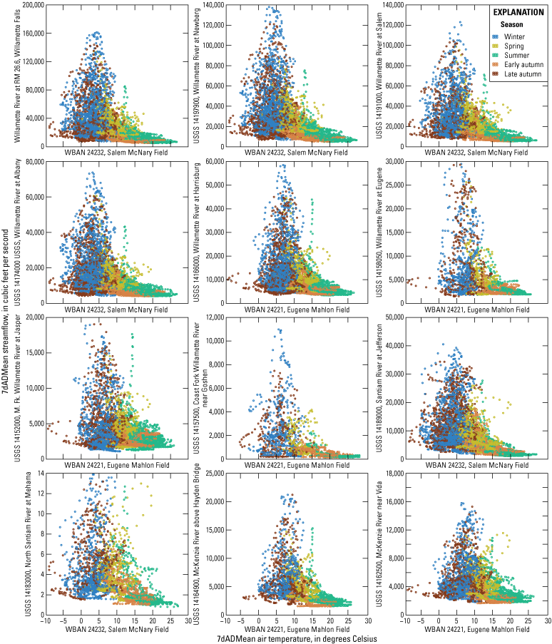
Graphs showing the source and range of the 7-day average of the daily mean (7dADMean) streamflow and 7dADMean air temperature data used to create each regression model. See table 1 for additional information on location and data sources and time periods included in regression models.
Conversion Factors
Temperature in degrees Celsius (°C) may be converted to degrees Fahrenheit (°F) as follows:
°F = (1.8 × °C) + 32.
Temperature in degrees Fahrenheit (°F) may be converted to degrees Celsius (°C) as follows:
°C = (°F – 32) / 1.8.
Datums
Vertical coordinate information is referenced to the North American Vertical Datum of 1988 (NAVD 88).
Horizontal coordinate information is referenced to the North American Datum of 1983 (NAD 83).
Elevation, as used in this report, refers to distance above the vertical datum.
Publishing support provided by the U.S. Geological Survey
Science Publishing Network, Tacoma Publishing Service Center
For more information concerning the research in this report, contact the
Director, Oregon Water Science Center
U.S. Geological Survey
2130 SW 5th Avenue
Portland, Oregon 97201
Disclaimers
Any use of trade, firm, or product names is for descriptive purposes only and does not imply endorsement by the U.S. Government.
Although this information product, for the most part, is in the public domain, it also may contain copyrighted materials as noted in the text. Permission to reproduce copyrighted items must be secured from the copyright owner.
Suggested Citation
Stratton Garvin, L.E., Rounds, S.A., and Buccola, N.L., 2022, Estimating stream temperature in the Willamette River Basin, northwestern Oregon—A regression-based approach: U.S. Geological Survey Scientific Investigations Report 2021–5022, 40 p., https://doi.org/10.3133/sir20215022.
ISSN: 2328-0328 (online)
Study Area
| Publication type | Report |
|---|---|
| Publication Subtype | USGS Numbered Series |
| Title | Estimating stream temperature in the Willamette River Basin, northwestern Oregon—A regression-based approach |
| Series title | Scientific Investigations Report |
| Series number | 2021-5022 |
| DOI | 10.3133/sir20215022 |
| Publication Date | May 12, 2022 |
| Year Published | 2022 |
| Language | English |
| Publisher | U.S. Geological Survey |
| Publisher location | Reston, VA |
| Contributing office(s) | Oregon Water Science Center |
| Description | Report: viii, 40 p.; Data Release |
| Larger Work Type | Report |
| Country | United States |
| State | Oregon |
| Other Geospatial | Willamette River Basin |
| Online Only (Y/N) | Y |