

Water-Quality Trends in the Delaware River Basin Calculated Using Multisource Data and Two Methods for Trend Periods Ending in 2018
Links
- Document: Report (16.2 MB pdf) , HTML , XML
- Related Work: USGS Fact Sheet 2023-3014 (html)
- Data Releases:
- USGS data release - Multisource surface-water-quality data and U.S. Geological Survey streamgage match for the Delaware River Basin
- USGS data release - Water-quality trends for rivers and streams in the Delaware River Basin using Weighted Regressions on Time, Discharge, and Season (WRTDS) models, Seasonal Kendall Trend (SKT) tests, and multisource data, water years 1978–2018
- Download citation as: RIS | Dublin Core
Abstract
Many organizations in the Delaware River Basin (DRB) monitor surface-water quality for regulatory, scientific, and decision-making purposes. In support of these purposes, over 260,000 water-quality records provided by 8 different organizations were compiled, screened, and used to generate water-quality trends in the DRB. These trends, for periods of record that end in 2018, were generated for 124 sites and up to 16 constituents using 2 trend methods: the Seasonal Kendall Test and the Weighted Regressions on Time, Discharge, and Season model. Seasonal Kendall Tests were performed on all water-quality records to detect monotonic trends in concentration over the period of record and for as many as four additional trend periods (1978–2018, 1998–2018, 2003–18, and 2008–18). The Weighted Regressions on Time, Discharge, and Season model was applied to water-quality records that passed more stringent screening criteria and was used to detect monontonic and nonmonotonic trends, account for variations in streamflow, and estimate annual concentrations. These two trend methods produced different trend directions less than 1 percent of the time, illustrating general agreement between the methods despite the different approaches and data input requirements. Overall, the changes in concentration for salinity constituents (specific conductance and total dissolved solids), chloride, and sodium were increases; those increases were some of the largest changes observed in the basin, and they occurred at faster rates over time. Total dissolved solids concentration trends at 4 of the 60 sites increased from below to above the level of concern threshold (a secondary drinking water threshold) over the period of record, indicating potentially meaningful degradation in water quality. Nutrient constituent (ammonia, nitrate, orthophosphate, total nitrogen, and total phosphorus) concentrations tended to decrease over the period of record, although fewer sites had significant trends and the changes in concentration were smaller compared to the salinity constituents. Total nitrogen and total phosphorus were the only nutrient constituents to have decreasing concentration trends that crossed from above to below the level of concern threshold, U.S. Environmental Protection Agency (EPA) ecoregional nutrient criteria, (EPA, undated c). This finding indicates water-quality improvement at sites with these trends (nine sites with total nitrogen trends and one site with a total phosphorus trend), although many sites were still in exceedance of the level of concern. Trends for total suspended solids and some major ions (calcium, magnesium, potassium) were largely nonsignificant or variable between sites, with no prevalent patterns across the DRB; however, sulfate concentrations decreased at most sites. Cumulative land-surface change within each watershed had a strong positive relation with changes in water-quality concentrations for the salinity constituents and most major ions, but not for the other constituents, indicating that land-surface changes are related to the sources and transport of these constituents. Investigating long-term trends (a decade or longer) in water quality can help the DRB water management community quantify the success of management practices and identify potential threats to water availability.
Introduction
The Delaware River Basin provides freshwater to 8.3 million people living in the basin and supports an additional 5 million people outside of the basin with drinking water. The Delaware River Basin also provides recreational opportunities to millions of residents and visitors every year, and its waters are essential for supporting ecological communities, industry, and transportation (Delaware River Basin Commission, 2019). Before the early 20th century, water quality of the Delaware River Basin had been degraded to the point of interfering with its use for human and ecological purposes. Over decades, the dedicated and coordinated efforts by Federal and State governments improved the quality of water throughout the basin (Kummer, 2020). Across the Delaware River Basin, a variety of water quantity and quality characteristics, including the populations of supported organisms, are now described as “good” or “very good” and have been “improving” or “stable” over time (Delaware River Basin Commission, 2019). Focus has shifted, therefore, from improving to maintaining and protecting this level of quality. With this goal in mind, many organizations in the Delaware River Basin monitor surface-water quality to track any changes in conditions that might warrant a change in how water quality is assessed, managed, or regulated. For example, one way water-quality trends in the Delaware River Basin are assessed is through the Delaware River Basin Commission Special Protection Water Program, which assesses “measurable change to existing water quality” (Delaware River Basin Commission, 2018).
The U.S. Geological Survey’s (USGS) Integrated Water Availability Assessments Program used the data collected by the Delaware River Basin Commission and other monitoring organizations to assess the status and trends of surface-water quality for 16 constituents at 124 sites across the Delaware River Basin, beginning as early as 1968. The objectives of this report are to describe the data processing, screening, and methods used to generate water-quality trends in the Delaware River Basin, using two trend methods, and to assess and summarize these trend results. This report contextualizes the changes in water quality by comparing trends to levels of concern (LOCs) and assessing the changes in relation to land use to make inferences about the potential drivers of these changes. This report also addresses some noted challenges of assessing trends in the Delaware River Basin, such as the need for many observations and the need to control for variability in water-quality conditions due to streamflow (Delaware River Basin Commission, 2016).
Incorporating data from monitoring organizations in addition to the USGS created a larger, richer dataset that expanded the number of sites available for trend analysis and produced denser water-quality records at some sites, leading to more accurate and well-characterized trends. Trends were determined for the longest period that met screening criteria for each constituent at each site, and for as much as four additional trend periods (1978–2018, 1998–2018, 2003–18, and 2008–18), depending on the length of record. This study used two trend methods to characterize changes in water quality in the rivers and streams of the Delaware River Basin: the Weighted Regressions on Time, Discharge, and Season (WRTDS) model (Hirsch and others, 2010; Choquette and others, 2019) and the Seasonal Kendall Test (SKT) (Hirsch and others,1982). WRTDS is a statistical model that estimates annual mean concentrations and loads and characterizes trends in these annual mean concentrations and loads over time. This methodology quantifies the uncertainty in trend estimates and produces outputs that allow for a rich understanding of changing water quality; however, it requires a complete daily record of streamflow to pair with water-quality data, which often restricts the number of sites where WRTDS can be used because many water-quality monitoring sites are not co-located with streamgages. The SKT is a statistical test for a monotonic relation between water-quality concentrations and time, and it can be paired with the calculation of the Theil-Sen slope to estimate a rate of change (Helsel and others, 2020). Compared to WRTDS, this approach is less robust and provides less information about how water quality changes over time. However, because the SKT requires only water-quality concentration data, it could be applied at more sites and for longer periods than WRTDS, improving our understanding of the spatial and temporal variability of trends in the Delaware River Basin.
Trends were summarized by trend method and constituent and investigated based on their direction, magnitude of change, rate of change, and their relation to LOCs established for human health and aquatic life. Additionally, trends were assessed based on land-use categorizations, land cover changes, and spatial distributions. Lastly, a comparison of the direction and magnitude of trends determined by the two different methods was completed, when trend estimation was possible for the same sites and constituents, so that trend analysts can more fully understand the advantages and drawbacks of the two techniques. The methodology presented here, built upon the work of Oelsner and others (2017), demonstrates how multisource data can be combined and how multiple trend techniques can be used to determine trends at more sites, for longer periods of record, and with more certainty than using data from a single agency or with a single method alone. By updating the workflow for using multisource data and calculating water-quality trends, this report revises the template for completing assessements that require similar data and analyses in other basins. To inform future management actions and monitoring efforts, there is a need to understand how water quality has changed over time. This analysis updates and expands the understanding of water-quality trends in the Delaware River Basin, highlights constituents of concern, and presents additional monitoring needs. This assessment can direct future research into the drivers of these trends and thus inform mitigation strategies to curb the effects of degraded water quality or provide evidence for management strategies that are successfully improving water quality.
Methods
To estimate changes in the water quality of rivers and streams in the Delaware River Basin, we used multisource data and two trend methods. Figure 1 illustrates the overall workflow described in detail in this section. First, multisource data were retrieved from the Water Quality Portal and “harmonized,” meaning that the data were refined to create a quality-controlled dataset with consistent nomenclature (Shoda and others, 2019a). From this harmonized dataset, water-quality constituents were selected, and the data for those constituents were further processed in preparation for trend analysis, as detailed in the section below. Then, monitoring locations were assessed to determine if and how water-quality data from these locations might be appropriately combined between multiple nearby locations in a process known as “site clustering.” Water-quality data were then screened for seasonal and temporal representativeness, and water-quality sites were paired with available USGS streamgages. Water-quality and streamflow data were then screened with more stringent criteria for appropriate estimation with WRTDS. Lastly, common trend periods were defined so that in some analyses, trends for different constituents and methods could be assessed for the same period.
The assessment described in this report implements many of the data processing steps and screens developed for the USGS’s national-scale water-quality trends assessment (Oelsner and others, 2017; Murphy and Sprague, 2019). One major divergence in this assessment from previous assessments is that water-quality data from multiple monitoring locations and collecting organizations were combined (“site clustering”). An additional difference described in this report is that water-quality records were screened to identify the longest period of record (POR) that passed various temporal and data density criteria, instead of screening with predefined trend periods. These changes gave this analysis more flexibility and allowed for broader incorporation of non-USGS data.
Water-quality trend estimations for all site-constituent combinations are in Murphy and others (2020). This section describes the detailed steps we followed to estimate water-quality trends, beginning with the harmonized dataset (Shoda and others, 2019a) and ending with two different estimating methods. All data processing, trend estimation, statistical testing, and data visualization for this study were performed using R software (version 3.6.3) and R Studio (Version 1.2.5033) (R Core Team, 2020). Data were retrieved using the dataRetrieval package (De Cicco and others, 2018). Data processing and modeling used the dplyr, tidyr, and ggplot2 packages (Wickham, 2016; Wickham and Henry, 2020; Wickham and others, 2020). All input data, R code, and output from this analysis, including concentration results from both trend methods and load results from WRTDS, are available in Murphy and others (2020).
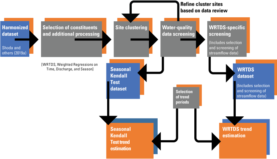
Diagram of the data processing workflow described in the “Methods” section.
Data Retrieval and Harmonization
Discrete surface-water-quality data for the Delaware River Basin were retrieved primarily from the Water Quality Portal, a national data repository which serves data collected by hundreds of Federal, State, and local organizations (National Water Quality Monitoring Council, 2019; Murphy and Shoda, 2020). Data were then harmonized in a process that includes steps such as: (1) selecting and combining appropriate water-quality constituent names; (2) identifying comparable and problematic methods; (3) standardizing text fields, such as lab remarks; (4) converting results to common units; (5) identifying proper fractionation; (6) assessing missing, zero, or unrealistic result values; (7) synthesizing remark codes and data quality comments; and (8) preferentially removing duplicate records. The purpose of this process was to combine data from multiple sources and create a reliable and comparable dataset for use in analysis and modeling (Shoda and others, 2019a). Many of these steps were based on the processes described in Oelsner and others (2017). A more detailed description of the data harmonization process for the Delaware River Basin dataset used in this analysis, including the R code used to retrieve and harmonize data, is available in Shoda and others (2019a). In addition to the data retrieved from the Water Quality Portal, data for 27 sites were obtained from the New York City Department of Environmental Protection for a subset of constituents. These data were harmonized following the same steps outlined in Shoda and others (2019a).
Selection of Water-Quality Constituents and Additional Data Processing
Four groups of constituents were chosen for trend assessment, based on their importance to Delaware River Basin stakeholders and the availability of existing guidance on data harmonization for these constituents. Salinity constituents were defined as specific conductance (SC) and total dissolved solids (TDS). The term “salinity” commonly refers to the dissolved salt content in water. It can be measured holistically with SC, which is directly related to the ion content of water, or by measuring TDS, which represents the ions and other dissolved solids in water. More specifically, the major ions that contribute to salinity (calcium, chloride, magnesium, potassium, sodium, and sulfate) can be measured directly and represent their own constituent group. In this report, salinity and major ions constituents are often discussed together because of their interrelated nature. Nutrient constituents were ammonia, nitrate, orthophosphate (filtered and unfiltered), total nitrogen (TN), and total phosphorus (TP), and suspended solids constituents were suspended sediment and total suspended solids (TSS).
For some constituents assessed in this study, data from filtered and unfiltered fractions were combined based on analyses in Oelsner and others (2017), who found a low percentage difference between the filtered and unfiltered concentrations of certain constituents in thousands of samples collected nationally, including in the Delaware River Basin. Oelsner and others (2017) combined data for samples with filtered and unfiltered fractions of ammonia, nitrate, nitrite plus nitrate, chloride, and sulfate. Although not all major ions analyzed for this report were directly assessed by Oelsner and others (2017), fractions were also combined for calcium, magnesium, potassium, and sodium. In contrast, the filtered and unfiltered fractions of orthophosphate were not suitable for combination and are referred to as separate constituents in this report. Table 1.1 lists the constituents and fractions used in this study and indicates which were combined. After this step, a few additional data processing steps were performed, including the selection of one value per site, constituent, and day (“data thinning”) and adjustments to censoring based on published technical memorandums. These steps are documented in appendix 1.
Site Clustering
The harmonized dataset contains water-quality data for 5,014 monitoring locations across the Delaware River Basin (Shoda and others, 2019a), each having at least one water-quality sample. Data from all locations were either combined to form “cluster sites” or used independently as single “sites” in this analysis. In general, each monitoring location has a unique identifier that is specific to a collecting organization and sampling location on a river or stream. However, some collecting organizations assign a new monitoring location identifier to the same sampling location to distinguish sampling for a new project or a different network. When multiple monitoring location identifiers are associated with the same location or when monitoring locations are closely located on the same river or stream, their sampling is capturing virtually the same streamflow and water-quality conditions. When appropriate, combining data from multiple monitoring locations can increase the length of record and (or) increase the data density within a record, both of which increase the robustness of the dataset used for the estimation of trends. Nevertheless, precautions must be taken when combining data from different collecting organizations. Data from one organization may be biased compared with the data from another organization, which could lead to an artificial trend in the data due solely to differences in sample collection or analysis procedures between the collecting organizations.
In this study, the term “site” describes a particular location or stretch of stream that may have data from a single monitoring location (“single site”) or from multiple nearby monitoring locations (“cluster site”). Data from multiple monitoring locations were considered for grouping into a cluster site if they were: (1) co-located (in other words, a collecting organization assigned more than one identifier to the same location or the same location on a river was monitored by more than one collecting organization); (2) on the same flowline, defined as a unique stream segment in the medium resolution National Hydrography Dataset V2 (McKay and others, 2012) (otherwise known as a ComID), and the flowline was less than 1.5 kilometer long; or (3) on the same flowline and the distances between monitoring locations were no more than 10 percent of the length of the flowline (fig. 2). In the third scenario, when many sites were on the same flowline, hierarchal clustering and a distance matrix were used to determine the best grouping of monitoring locations. The greatest distance between any two sites in a cluster was 1.6 kilometers.
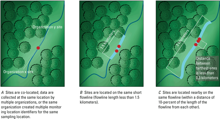
Three scenarios in which water-quality data from A, the same location; or B and C, nearby locations on the same flowline were considered for combination in subsequent analysis (in other words, criteria for creating a “cluster site”). Note: not to scale.
Cluster Sites Refined Based on Data Review
The specific monitoring locations that were included in each cluster site were refined by visually assessing the combined water-quality data. For each constituent at each cluster site, diagnostic plots including a cumulative distribution function plot, jitter plot, and a time series of the concentration data, color coded by the monitoring location identifier, were reviewed. During review, specific monitoring locations were flagged for exclusion from a cluster site if the data appeared to be discordant with the other monitoring location(s), particularly if combining the data appeared to induce an artificial trend. These reviews were constituent-specific, thus for the same cluster site, a monitoring location may be excluded from the dataset for one constituent but be included for a different constituent. This decision was considered acceptable because water-quality constituents differ in their response to variations in river morphology, riparian conditions, streamflow, and other factors. Factors that affect the concentration of one constituent might be less important for another. Furthermore, if differences were due to sample collection or laboratory procedures, these may also only affect certain constituents at a given cluster site (Martin and others, 1992).
Additionally, all cluster sites were evaluated with aerial imagery for intervening influences that could lead to differences in water-quality conditions between monitoring locations. Intervening influences were defined as major dams or National Pollutant Discharge Elimination System dischargers and were not allowed to be between monitoring locations in a site cluster. Murphy and others (2020) includes a table that lists which monitoring locations contributed data to each cluster site, for each constituent. Each site was assigned a unique identifier, which was used in all subsequent data processing and trend analysis.
Data Screening
Data for all sites and constituents were screened following the steps described in this section (each site-constituent combination is hereafter referred to as a water-quality record). All water-quality records that passed the screening described in the following “Water-Quality Data Screening” section had trends estimated with the SKT. Those records that passed additional screening described in the “WRTDS-Specific Screening” section also had trends estimated with WRTDS.
Water-Quality Data Screening
Site-specific data for the 16 constituents noted previously were then screened for their suitability for SKT and WRTDS trend analyses. The goal of screening each water-quality record was to ensure that the data met a basic set of criteria for representative sampling, which allows for robust trend analysis. The criteria used were developed to ensure that the seasonal and temporal characteristics at a site were adequately represented by the existing water-quality data. Three of the five criteria assess the presence of at least quarterly samples. Following Oelsner and others (2017), the water year was divided into quarters three different ways, and water-quality samples were required to meet at least one of the three quarterly definitions. Flexibility in the definition of which months compose a quarter of a year accommodates variations in sample collection schedules due to issues such as freezing. Oelsner and others (2017) provides more information in their “Coverage of Changing Seasons” sections and table 4 of the same work.
The following criteria were used to screen water-quality data.
-
• End-year criteria—At least 2 water years with quarterly samples are required in a 3-year window that includes the end year of the trend period and the two preceding years. For this study, the end year of the trend was 2018; therefore, 2 years with quarterly samples were required in 2016–18.
-
• Start-year criteria—Quarterly samples are required in the start-year and in at least 1 of the next 3 years (in other words, at least 2 years with quarterly samples are required in a 4-year window, one of which must be the start year). For example, for a water-quality record starting in 1970, quarterly samples would be required in 1970 and in one of the following years: 1971, 1972, or 1973.
-
• Data density criteria—Between the start and end years of the water-quality record, at least 70 percent of the years must have at least quarterly samples.
-
• Gap-length criteria—The water-quality record can have a maximum of 5 consecutive years with less than quarterly samples.
-
• Minimum length criteria—The water-quality record must be at least 10 years long. For this study, because 2018 was the target end year, the minimum start year must be 2009 or earlier.
Each water-quality record was evaluated for these criteria in an iterative process, by water year, starting with the earliest water year with quarterly samples. This process results in the longest possible timeframe in which all criteria were met. The criteria used in this study are based largely on the criteria in Oelsner and others (2017); however, they differ in a few important ways. Oelsner and others (2017) screened water-quality records by prespecified trend periods, allowing for gaps of any length in the middle of the trend period, as long as the criteria at the start and end of the period and the temporal screening criteria were met. The advantage of this approach is that allowing for data gaps increases the number of sites and constituents that meet the data screening, therefore, allowing more data into the analysis but having no negative effect on the strength of the analysis to detect changes in water quality between the start and the end of the defined trend period. The disadvantage of this approach is that because there are sometimes substantial gaps in the water-quality record, the period between the start and end of the trend period cannot always be assessed reliably. In this study, trend periods were not used in data screening. As discussed previously, the longest POR meeting the screening criteria was identified for each water-quality record. By screening this way, we can be confident in the generation of a representative record, and changes can be determined between any two points in time. Thus, in addition to using a POR trend, four additional trend periods were selected after data screening as described later in this report.
WRTDS-Specific Screening
Because WRTDS uses streamflow data to estimate trends, trend estimation with this methodology required each water-quality site to be matched to a USGS streamgage. Water-quality sites and streamgages were indexed to National Hydrography Dataset flowlines, and each water-quality site was evaluated for a match to a streamgage on the same, or nearby flowlines. When a streamgage was not present on the same flowline as a water-quality site, streamgages with drainage areas that were no more than 10 percent different from the drainage area of the water-quality site were considered potential matches. Shoda and others (2019a) provides these initial one-to-many streamgage matches. Streamflow data from these potential streamgage matches were retrieved from the National Water Information System (USGS, 2019) using the dataRetrieval package (De Cicco and others, 2018). Streamflow records were required to meet the following criteria, based on the screening developed by Oelsner and others (2017):
-
• no more than 30 days of missing streamflow per year,
-
• no more than 3 consecutive days of missing streamflow per year,
-
• no days of negative streamflow, and
-
• no more than 30 days of zero streamflow per year.
Zero streamflow values were substituted with a small constant, and small gaps in streamflow data were interpolated following Oelsner and others (2017). For trend estimation with WRTDS, each water-quality site was required to match a single streamgage that met the above criteria. When multiple streamgages were matched to a water-quality site, streamgage selection was based on POR length and proximity to the site, following the procedure provided in Oelsner and others (2017). When the streamgage POR was shorter than the water-quality POR, the water-quality POR was shortened until the water-quality site and streamgage match met all screening criteria and shared the same POR. Lastly, all potential water-quality site and streamgage matches were manually reviewed for intervening influences (defined previously) that would cause streamflow to differ substantially between the site and the streamgage. For matches in which the water-quality site and streamgage were on different flowlines, the streamgage data were scaled by multiplying each discharge value by the ratio of the water-quality site drainage area to the streamgage drainage area, following the procedure by Oelsner and others (2017).
In addition to ensuring the water-quality data were representative of seasonal and temporal conditions, we also verified that the water-quality data were collected across the range of streamflow conditions at a site, in particular high streamflow. Without adequate sampling during high streamflow, the water-quality concentrations and loads during these flows are unknown, and thus are extrapolated by the WRTDS model. Extrapolation of any model beyond its calibration data can result in increased uncertainty and bias. This is especially problematic for some constituents, such as suspended sediment, TSS, and TP that have most of their annual load transported during high streamflow conditions, and without data to represent these conditions, these extrapolated estimates can be unreliable.
In Oelsner and others (2017), high-flow conditions were characterized for each decade by the 85th percentile of flows during each month at a streamgage, and trend periods (based on decades) were required to have a certain percentage of samples collected during these high-flow conditions. As described previously, we did not define trend periods before water-quality and streamflow screening, so we modified the approach used by Oelsner and others (2017) to assess sample coverage during high streamflow conditions in the following way. The length of the POR at each site was divided into the largest possible number of subperiods that were equal to or greater than 10 years and of the closest possible equal length (in whole years). For example, a POR of 25 years would be divided into subperiods of 12 and 13 years. Then, the number and percent of samples collected above a given flow magnitude were determined; these are referred to as “high flow samples.” This approach ensures that samples collected during high flow are distributed throughout the trend POR. Defining “high flow” as the 85th percentile of flow for each month of each subperiod, at least half of the subperiods were required to have at least 14 percent high-flow samples, or 20 high-flow samples, and the other subperiods were required to have at least 10 percent high-flow samples. The percentage criteria (at least 14 percent) follows the high-flow screen in Oelsner and others (2017), but for this analysis, we added an additional high-flow sample count criteria because at some sites there was robust sampling during high-flow conditions (for example, greater than 20 high-flow samples were collected); however, the high-flow sample percentages did not meet the criteria due to the large total number of samples. Finally, at least 50 percent of the screened water-quality records were required to contain quantified concentrations (uncensored data). Only water-quality records meeting these additional criteria were analyzed with WRTDS.
Selection of Four Common Trend Periods
As described previously, each water-quality record was required to meet the water-quality screening criteria, and the length of the POR was allowed to vary for each water-quality record. A POR trend was determined for each water-quality record using the earliest and latest year of the record that met the screening criteria. There was not a clear or obvious policy implementation or other change point to target for assessment in the Delaware River Basin, and the approach used in this report allows for an understanding of how conditions changed over the longest possible period. For some assessments, however, there is a need to compare trends for the same periods. Therefore, trends were also determined for four additional trend periods, as available data allowed: 1978–2018, 1998–2018, 2003–18, and 2008–18. These four trend periods were determined using an approach that maximized the number of sites and the length of record for all constituents. In a precedent set by Oelsner and others (2017) with the intent to include as many sites and constituents as possible for each trend period, we allowed screened water-quality records ending 1 year earlier than the end of the trend period (2017) and (or) beginning one year later than the defined start of the periods (1979, 1999, 2004 and 2009) to be considered. As such, the WRTDS results for some sites and constituents have start or end years that vary by 1 year for these four trend periods. Because of this 1-year variation allowance for WRTDS results, all SKT trends were run using 1979, 1999, 2004 and 2009 as start years for the four trend periods, though for ease of interpretation, we refer to the trend periods as 1978–2018, 1998–2018, 2003–18, and 2008–18. The results section of this report focuses only on the concentration trends for the POR and the most recent trend period (2008–18), with results for the remaining trend periods available in Murphy and others (2020).
Trend Estimation
A parametric and nonparametric trend estimation technique were each used in this analysis, and each had related strengths and weaknesses. The WRTDS trend estimation methodology is a parametric test that provides a host of outputs to understand the evolving nature of water quality, including daily, seasonal, and annual estimates of water quality; diagnostic tools to characterize water-quality trends through time; uncertainty estimates for trends and annual estimates; and techniques to explore relations between concentration and streamflow. Furthermore, WRTDS can accommodate data with multiple censoring levels and variations in sampling frequency. The power of this technique is accompanied by a need for streamflow data and water-quality samples collected during high-flow conditions, which often limit the applicability of this method. The SKT is a nonparametric test and compared with WRTDS, the SKT and the Theil-Sen slope become less robust with increasing amounts of censored data, cannot accommodate multiple censoring levels, provide no information about the evolving patterns of change through time, and do not explore how concentrations relate to streamflow, which lead to reduced accuracy and power of the test (Hirsch and others, 2010). However, SKT trend estimates are widely applicable due to having less stringent data requirements and requiring less computing power and expertise to execute.
SKT Trend Estimation
For each water-quality record, the SKT was used to test for trends in water-quality concentration over the POR and for as many as four of the additional trend periods noted previously. The SKT is an extension of the Mann-Kendall test, testing for monotonic changes when there is an expected effect of seasonality (Hirsch and others, 1982). The SKT uses the Tau statistic, a nonparametric measure of correlative strength ranging from −1 to 1, indicating a stronger negative or positive trend as the Tau value approaches −1 or 1, respectively (Hirsch and others, 1982). The magnitude of change was determined using the Theil-Sen slope, which is a representation of the median slope of all pairwise comparisons through the data (Helsel and others, 2020).
Some additional data processing was required before running the SKT on concentration data for each water-quality record and trend period. If the data had multiple reporting levels, all data were recensored to the highest reporting level. The most common seasonal definition used during data screening (see previous) was used to define seasons for the SKT to create a dataset in which there is only one value per season. In this process, if there was a single result for a given season and year, that value was used. If there were multiple results, then the median value for that season, determined with the flipped Kaplan-Meier method, was used (Helsel, 2012). Finally, if more than 80 percent of the seasons in the trend period were censored values, the SKT was not run, following Oelsner and others (2017), and only the median concentration of the trend period was reported in the final output. If more than 40 percent but less than or equal to 80 percent of the seasonal data in the trend period were censored, then only the Tau statistic was reported. Estimates of the Theil-Sen slope become unreliable when a large percentage of the water-quality record is censored, while the Tau statistic is more robust to censored data. For these records, a significant increasing or decreasing trend can be identified, but the magnitude of the trend cannot be reliably quantified. If less than or equal to 40 percent of the seasons were censored, then the Tau statistic and the Theil-Sen slope were reported (Murphy and others, 2020). The SKT was performed using the smwrQW and smwrBase R packages (Lorenz, undated; Lorenz, 2015).
WRTDS Trend Estimation
In addition to the SKT, a subset of water-quality records that were paired with a USGS streamgage and passed additional screening (described previously) had trends also estimated using the WRTDS model (Hirsch and others, 2010). As its name suggests, WRTDS uses time, discharge, and season in a locally weighted regression to predict daily water-quality concentrations and loads. These daily values are aggregated to estimates of annual mean concentration and load for each water year throughout the POR. Flow-normalized (FN) estimates are also available, providing a characterization of the long-term change in concentration and load over time. The FN estimates of concentration and load remove the effects of random year-to-year variability in streamflow (Hirsch and others, 2010) but retain the effect of long-term changes in streamflow (referred to as generalized FN in Choquette and others, 2019). These FN estimates provide information about the evolving nature of water quality, capturing nonmonotonic trends over time. Changes in concentration and load for each trend period were calculated by subtracting the annual mean FN value at the end of the period from the annual mean FN value at the start of the period. Confidence intervals for the annual FN values and for the change between the start and end of the trend period were generated using a block bootstrap approach (Hirsch and others, 2015; Hirsch and others, 2018a). Lastly, the 2018 extension of the WRTDS method (Hirsch and De Cicco, 2018; Hirsch and others, 2018b Hirsch and others, 2018a) allows the resulting trend to be conceptualized as the sum of two components of change: change in water quality attributed to streamflow trends and change attributed to other changes in the watershed, such as management activities and decisions, constituent source availability, and transport through the watershed (Choquette and others, 2019; Murphy and Sprague, 2019). Detailed explanations of the WRTDS method, including the underlying concepts and statistical processes of the method, are available in Hirsch and others (2010); Hirsch and De Cicco (2015); Hirsch and others (2015); Oelsner and others (2017); Hirsch and others (2018b); Hirsch and others (2018a); and Murphy and Sprague (2019).
WRTDS was run on Yeti, the USGS supercomputer at the Denver Federal Center in Colorado (USGS, undated a). A WRTDS model was calibrated for each water-quality record separately using the entire POR. Model output included annual estimates of concentration and load, corresponding annual FN estimates, change estimates for each of the trend periods, and uncertainty estimates for the latter two result types. Results for each trend period were extracted from the single calibration (as opposed to rerunning WRTDS for each trend period). The R packages EGRET and EGRETci were used to run WRTDS (Hirsch and De Cicco, 2015; Hirsch and others, 2018b Hirsch and others, 2018a). Model specifications follow those of Oelsner and others (2017) and Murphy and Sprague (2019) and are available for each water-quality record in the associated data release (Murphy and others, 2020). The weighted regression half-window widths were set to 7 and 0.5 years for time and season, respectively, and two log cycles for streamflow. The minimum number of observations required for each weighted regression was defined as the smaller of either 100 observations or 75 percent of all observations. The minimum number of uncensored observations was set to one-half of the minimum number of observations. The edgeAdjust option was set to TRUE (to prevent overfitting of the model near the beginning and end of the record), bootBreak (minimum number of replicates) and nBoot (maximum number of replicates) were set to 100, and blockLength (block length for bootstrapping, in days) was set to 200. Following the guidance on model review outlined in Hirsch and De Cicco (2015) and further developed by Oelsner and others (2017), model diagnostics were reviewed. This review included a visual evaluation of plots of the residuals, observed data, and model estimates. Individual output for all modeled water-quality records that passed model review are available in Murphy and others (2020).
Evaluation of Trends
To better understand water-quality trends in the Delaware River Basin, results were evaluated in several ways. First, trends determined with SKT and WRTDS were assessed to understand their direction, magnitude, and rate of change. Second, the trends were compared to water-quality LOCs to contextualize the changes and understand their environmental significance. For trends that were increasing or decreasing towards a LOC, proximity to the LOC was assessed, and the rate of change was projected into the future to assess the potential timeframes required to cross above or below the LOC, respectively. Third, trends were summarized by land use and the change in land cover within each watershed, and general spatial patterns of the trends were evaluated. Lastly, when SKT and WRTDS could be applied to the same water-quality records, the two methodologies were directly compared.
In this report, the results of only one method (SKT or WRTDS) for each site, constituent, and trend period are presented. When WRTDS results were available, they were used preferentially to SKT results because WRTDS provides more detailed output and accounts for the effects of streamflow on changing water quality. In the analyses in which SKT and WRTDS results are presented side-by-side, the SKT trends are referred to as “unadjusted” to remind the reader that they differ from the FN trends generated by the WRTDS model. Most analyses in this report are for the POR trends; a few analyses summarize more current changes, and these use the most recent trend period of 2008–18. Additionally, there was only one site that passed the screening to calculate trends for suspended sediment concentration, so those results are not included in the summaries below but are available in Murphy and others (2020).
Trend Direction and Magnitude
Trend directions were defined as “increasing,” “decreasing,” and “nonsignificant,” using a p-value less than or equal to 0.1 to define the level of significance. To understand the magnitude of significant increases and decreases for the POR trends, the percentage change was calculated for each constituent and trend method for which there was a significant trend. The calculation of percentage change is the difference between the annual concentrations of the end year and start year divided by the start-year concentration and multiplied by 100. For the WRTDS results, percentage change was calculated using the estimated FN annual mean concentrations of the start and end years. For the SKT trends, percentage change was calculated by first estimating the start-year and end-year concentrations. The end-year concentration was calculated as the median concentration of the two most recent years of samples (for example, 2017 and 2018), and the start-year concentration was determined by projecting the Theil-Sen slope back from this end-year concentration to the earliest year in the POR. This approach for calculating start- and end-year concentrations by using the slope of the Theil-Sen line and the median concentration of the last 2 years of the record to determine the intercept of the line, better characterizes potential nonlinear changes compared to the more common approach (Helsel and others, 2020) of using the median concentration and median year of the trend period to determine the intercept (fig. 3). In the two cases in which this approach generated a negative start-year concentration, the lowest nonnegative estimated start concentration was used.
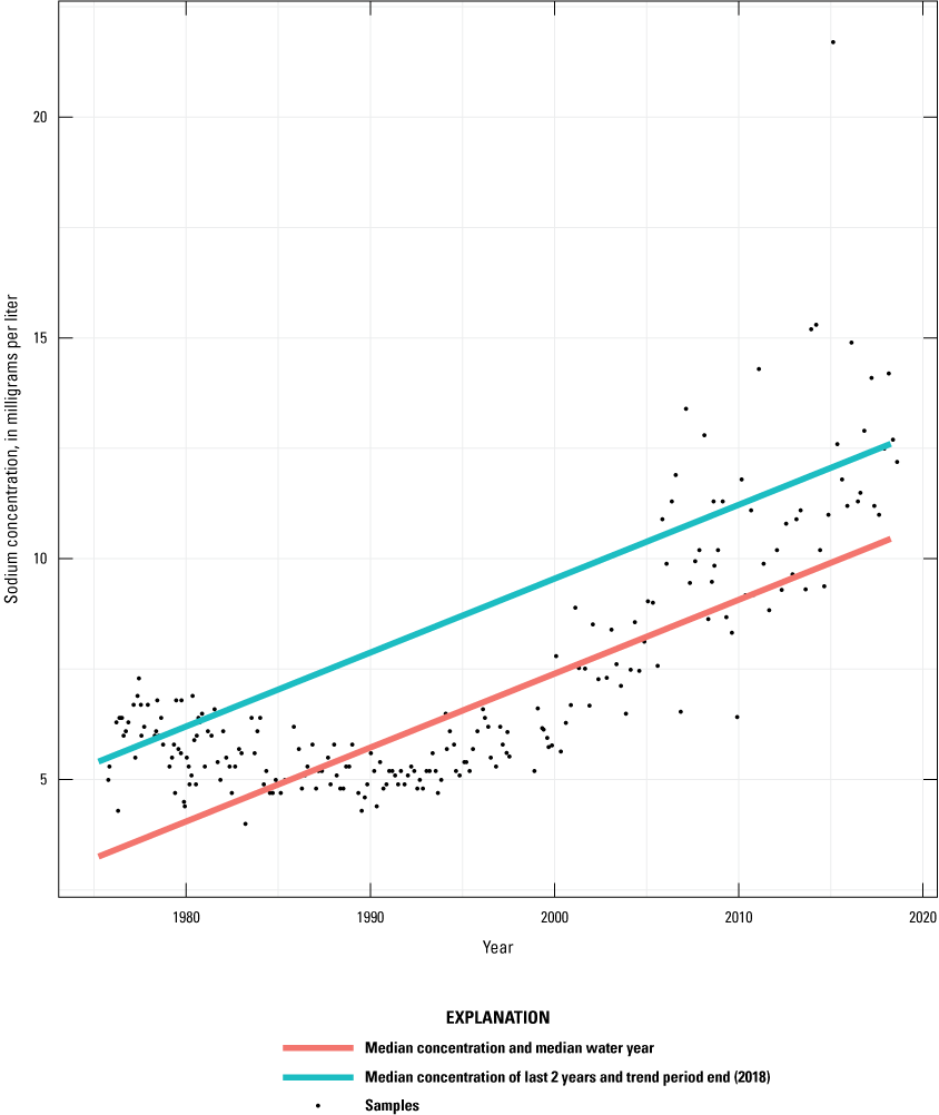
Example of trend lines for sodium at site cx_USGS-01411500 with the intercept of the Theil-Sen line determined with two approaches, using (1) the median concentration and the median year of the trend period, and (2) the median concentration of the last 2 years and the last year of the trend period.
Rate of Change Investigation
To characterize the temporal evolution of changing water quality across the Delaware River Basin, 5-year rates of change were calculated using the annual mean FN concentration estimates at sites with WRTDS results and compared between constituents and over time. This analysis does not include SKT results because the SKT does not model annual concentrations, and so it is not possible to calculate reliable rates of change for periods shorter than the POR. Considering only constituents that had trends estimated at more than 10 sites over the POR, rates of change in concentration were calculated for each site for the 4 constituents with the largest percentage of increasing POR trends and the 4 constituents with the largest percentage of decreasing POR trends. Rates were generated for every 5-year subperiod beginning in 1993 and ending in 2018 (1993–98, 1998–2003, 2003–08, 2008–13, and 2013–18) by subtracting the annual mean FN concentration for the start year from the end year’s annual mean FN concentration. For the selected constituents, these 5-year rates of change were pooled across sites that had significant POR trends in the selected trend direction, and the median and interquartile ranges (IQR) were calculated.
Level of Concern Comparisons
To understand the environmental significance of the water-quality trend, the annual mean concentrations for the start and end years were compared to water-quality levels of concern (LOCs), following Shoda and others (2019b). For the WRTDS results, the estimated FN annual mean concentrations of the start and end years were used. For the SKT results, the start-year and end-year concentrations were estimated as described in the previous section. A LOC is defined as a threshold value above which the threat of an undesirable effect exists for human health or aquatic life. The LOCs were compiled from various EPA sources and are listed in table 1. With the exception of the LOC for nitrate, these thresholds are nonregulatory and include maximum contaminant levels, secondary maximum contaminant levels, a taste threshold, and ecoregional nutrient criteria. These LOCs are suitable to compare to annual mean concentrations, as explained in Shoda and others (2019b). Comparisons were made for trends determined with both methods for sulfate, nitrate, ammonia, chloride, TDS, TN, and TP. The goal of these comparisons was to provide an environmental context for observed trends and to enrich our understanding of changing water quality. Because the trends reported in this study are for untreated water in rivers and streams, these comparisons are not intended to inform regulatory compliance or define eutrophication status, as discussed in Shoda and others (2019b).
Table 1.
Levels of concern for each constituent.[LOC, level of concern; mg/L, milligram per liter; EPA, U.S. Environmental Protection Agency; TDS, total dissolved solids; TN, total nitrogen; TP, total phosphorus]
Trend results were sorted into eight categories based on the trend direction and whether the trend start-year and end-year concentrations were above or below the LOC. Trends that crossed the LOC over the course of the POR were highlighted regardless of their trend significance because of the important water-quality implications that they represent. In this analysis, we used the POR trends because we wanted to characterize long-term changes relevant to human and aquatic life in the Delaware River Basin and assess the longest possible period over which environmentally significant change might have occurred. LOC comparison results for the most recent trend period (2008–18) are provided in the appendix (fig. 1.3).
To investigate the most recent trajectories of change, the significant 2008–18 trends that were approaching the LOC were examined further. First, the proximity of end-year concentrations to the LOC was explored for increasing trends that were approaching the LOC from below (in the “below LOC, increasing” category) and for decreasing trends that were approaching the LOC from above (in the “above LOC, decreasing” category), following Shoda and others (2019b). For each constituent and trend direction, end-year concentrations were sorted into 1 of 5 cells representing proximity to the LOC, with each cell increasing in value away from the LOC in intervals of 20 percent of the LOC. The use of cells to show proximity to the LOC allows for an intuitive visualization of how close or far the trend end-year concentrations were from the LOC.
Lastly, for the 2008–18 trends that were approaching the LOC, the change between the start- and end-year concentrations were used to calculate a rate of change (in milligrams per liter per year). This rate was projected into the future to determine the number of years it would take concentrations of the selected constituents to reach the LOC. These estimates of projected years to reach the LOC are intended to describe the magnitude of the trend results, not to predict concentrations in the future, because it is uncertain if these rates of change will hold constant for extended periods of time, and many factors contribute to trends and fluctuations in water quality.
Land Use and Spatial Summary
Lastly, trend results were summarized by watershed land-use categorizations, by a metric of land cover change, and assessed by geographic distribution. Land Change Monitoring, Assessment, and Projection (LCMAP) data (Zhu and Woodcock, 2014; Brown and others, 2020) were used to determine land-use categorizations and derive a metric of cumulative change for each watershed for years spanning 1986 to 2017. Each pixel of the LCMAP product contains a primary land cover classification and when aggregated, these were used to classify watersheds as urban (greater than 25 percent urban and less than 25 percent agriculture), agricultural (greater than 50 percent agriculture and less than 10 percent urban), undeveloped (less than 5 percent urban and less than 25 percent agriculture), or mixed (everything that does not fit in one of the above categories), following Stone and others (2014). The cumulative land-surface change metric was based on the LCMAP product Time of Spectral Change, which determined for each pixel whether land cover changed on a particular day of the year. These land cover changes can be large and possibly permanent or subtle and transient. For each year and site, the percentage of the watershed that changed was calculated as the sum of the number of pixels that changed at least once during a given year, divided by the total number of pixels constituting the watershed, multiplied by 100. These annual percentages were summed across the POR (starting in 1986 or the earliest year of each water-quality record) and for the most recent 10-year period (2008–17) and then plotted against the POR and 2008–18 water-quality trends, respectively. This metric gives a measure of the cumulative land-surface change in a watershed over a specified period of time, as a percentage of the watershed. Technically, this number can be greater than 100 percent if large parts of the watershed experienced land-surface changes repeatedly over multiple years. This metric does not specify how the land surface changed but does indicate whether there was a change. Importantly, this metric captures large and small disturbances to the land surface, including those that do not result in a change in land-use categorization. Examples of changes in the land surface that might not change land-use categorization include the intensification of development, destruction of infrastructure and vegetation due to natural disasters (for example, tornados, hurricanes, or forest fires), thinning of a forest due to selective harvesting or insect infestation, a large and extensive snowfall, or drought-caused extensive drying to grasses. LCMAP data products are described in further detail in Zhu and Woodcock (2014) and Brown and others (2020). Finally, maps were created to show the geographic distribution of trend patterns for each constituent. Maps were visually assessed for spatial patterns in trend direction and magnitude.
WRTDS and SKT Comparison
For a subset of sites, constituents, and trend periods, the criteria to use both SKT and WRTDS were met, and trend results were generated with both methods. An analysis of the comparability of trends determined with both methods was conducted when they were calculated for the same water-quality record and trend period. Because PORs could vary between methods for the same water-quality record, POR trends were excluded from this analysis, and only trends assessing the same trend periods were used. Trend directions during these trend periods were compared by calculating the percentage of paired trend analyses that fell in one of the following three groups: results that agreed between methods (significant trends in the same direction or nonsignificant trends), results in which significant trends had opposite directions, and trends in which one method found a significant trend and the other did not. In addition to assessing the comparability of trend direction, when trend direction results agreed and were significant, the magnitude of the water-quality change was compared by assessing the absolute value of the difference between the percentage changes determined by both methods.
Results
The final datasets of trend results generated in this analysis are published in Murphy and others (2020) and visualized on the “Tracking Water Quality in U.S. Streams and Rivers” web page (USGS, undated b). These datasets provide SKT results for every site, constituent, and trend period that met the water-quality data-screening criteria described above, and WRTDS results for a subset of sites, constituents, and trend periods that also met the more intensive WRTDS-specific criteria and had models that passed review. The datasets also include load estimations, trends in loads, and water-quality trend components for WRTDS results, which will not be discussed in this report. The following sections focus primarily on the concentration trends for the POR, with some discussion of the most recent 10-year trend period (2008–18).
Description of Trend Estimations
Eight collecting organizations contributed water-quality data to the input dataset published in Murphy and others (2020), and each organization contributed data for between 1 and 16 constituents. The sizes of these contributions varied; organizations contributed between 1 and 2,128 data values per site and constituent. Overall, non-USGS organizations contributed about half of the water-quality data values to the input dataset. In addition to direct data contributions, other organizations often partner with the USGS to fund, or partially fund, water-quality and streamflow data collection that is executed by the USGS. In the final trend results dataset described extensively in this report (1 trend per site, constituent, and trend period), each organization contributed water-quality data to between 3 and 797 water-quality records that met data-screening criteria (table 2). Of the 1,160 POR trends, about a third (345) were generated with water-quality data from more than one organization.
Table 2.
Collecting organizations that contributed data to the trend results discussed in this report, and the number of water-quality records that each organization supported.There were 124 sites in the Delaware River Basin that passed the water-quality data screening for at least one constituent (fig. 4). Streamflow data from 57 USGS streamgages were used in WRTDS trend estimation, and 59 sites passed the additional WRTDS screening for at least one constituent. Many sites have trend results for multiple constituents with results from SKT, WRTDS, or both. It is common that at the same site, the length of water-quality records and the quality of those records differ between constituents. Thus, trend results are specific to each site, constituent, trend period, and method. As stated previously, only the results for one method were used per constituent, site, and trend period in this report, and WRTDS was used preferentially over SKT. The number of sites with POR trends varies depending on the method used and the constituent (table 3).
Table 3.
The number of sites with period of record trends per constituent and trend method.[SKT, Seasonal Kendall Test; WRTDS, Weighted Regressions on Time, Discharge, and Season]
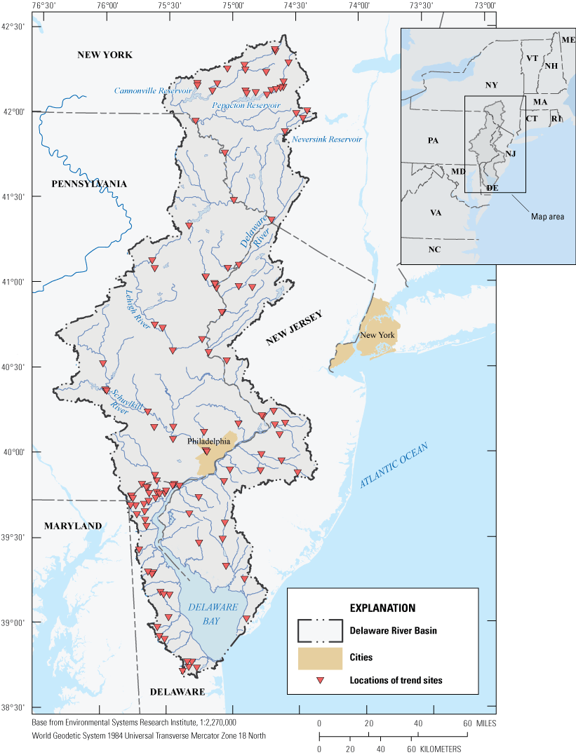
Sites with Weighted Regressions on Time, Discharge, and Season or Seasonal Kendall Test trends for at least one constituent.
For most constituents, trend sites were generally well distributed across the basin, but several constituents have a dense cluster of sites in northern Delaware (figs. 1.5–1.19). The geographic distribution of trend sites, however, was directly related to the organizations that contributed data to this analysis and where their monitoring programs were, so some constituents are less well distributed. The New York City Department of Environmental Protection, for example, monitors the upper Delaware River Basin at sites upstream from some reservoirs that provide drinking water to New York City, and they are one of the few organizations that contributed filtered orthophosphate data, therefore sites with trends for filtered orthophosphate were exclusively in the northernmost part of the basin (fig. 1.10). Likewise, the USGS Pennsylvania Water Science Center was the only organization that contributed unfiltered orthophosphate data that passed the screening, therefore sites with these trends are only in Pennsylvania (fig. 1.11). Murphy and others (2020) contains details on which organizations contributed data for which constituents and sites. Sites with TDS trends are not in the upper Delaware River Basin (fig. 1.16), and sodium and potassium trends were generally not west of the main stem of the Delaware River (figs. 1.14 and 1.12). Sodium, in particular, had only three sites in the Lehigh and Schuylkill River subbasins (fig. 1.14).
Period of Record Trend Direction and Magnitude
Overall, the significant POR trends for nutrients (orthophosphate, TN, nitrate, TP, and ammonia) tended to be mostly decreasing, and the significant trends for the salinity constituents (SC and TDS) and some major ions (sodium, chloride, and calcium) were largely increasing (fig. 5). For both trend methods, the constituents with the largest percentage of sites with increasing trends over the POR were indicators of salinity: SC, TDS, sodium, chloride, and calcium (fig. 5). Likewise, for both methods, the largest percentage of decreasing trends were observed for sulfate, orthophosphate (filtered and unfiltered), and TN (fig. 5). TSS, ammonia, and TP shared the largest percentage of nonsignificant trends for both methods (fig. 5). Potassium and magnesium shared a fairly even distribution of sites with increasing, decreasing, and nonsignificant trends for both methods. Overall, the WRTDS and SKT trend results were largely in agreement, although for calcium, magnesium, nitrate, potassium, and unfiltered orthophosphate the trend direction with the largest number of sites was not consistent between methods, and the highest percentage of sites was nonsignificant for one method and significant for the other method.
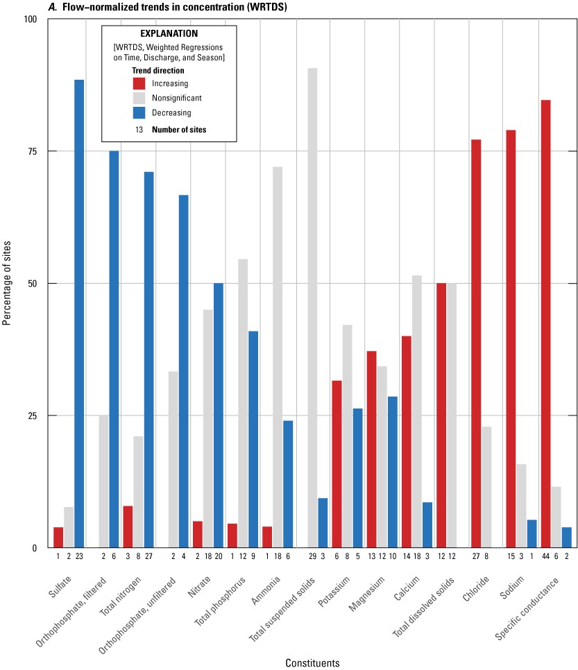
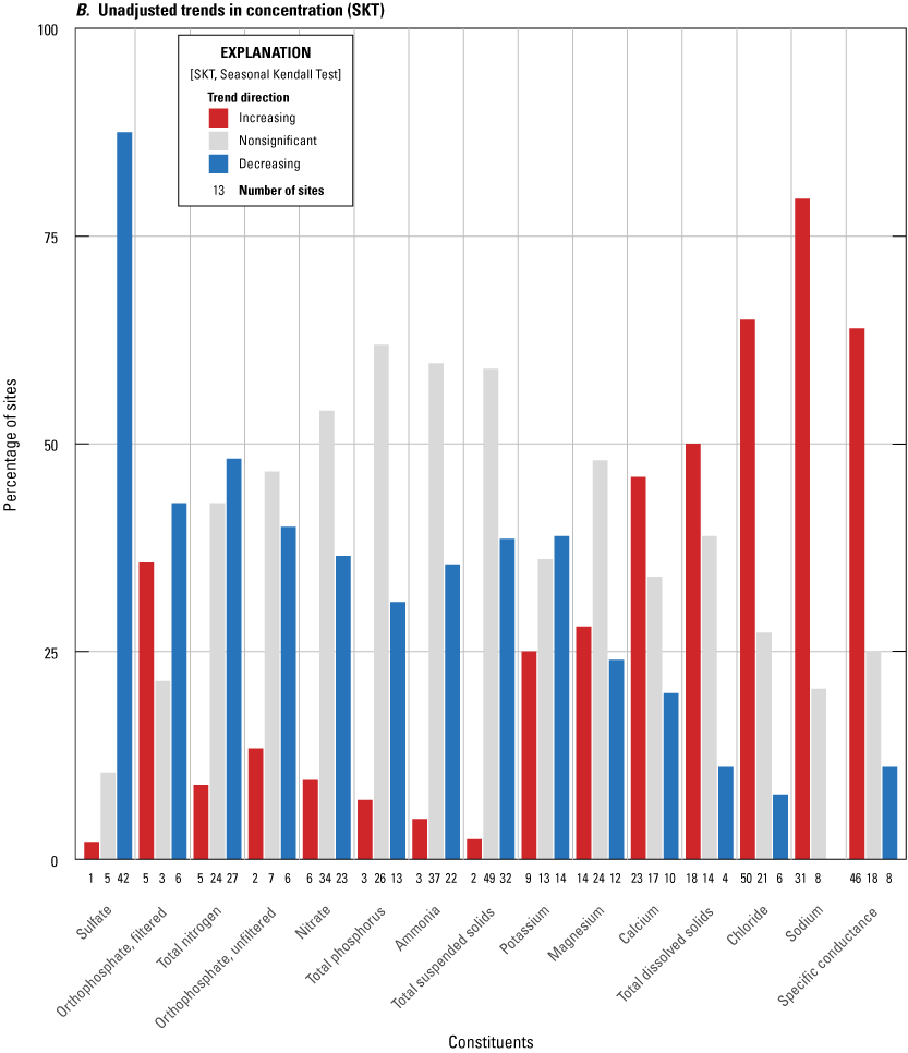
Percentage of sites with increasing, nonsignificant, and decreasing trends for each constituent for the period of record for A, flow-normalized trends in concentration calculated with Weighted Regressions on Time, Discharge, and Season and B, unadjusted trends in concentration calculated with the Seasonal Kendall Test.
Trend magnitudes followed a pattern similar to trend directions: the largest positive changes were for salinity constituents, chloride, and sodium and some of the largest negative changes occurred for nutrient constituents (fig. 6). For both methods, chloride, sodium, TDS, SC, calcium, and magnesium had the largest positive median percentage changes: their values ranged from 10 percent to 78 percent. Nutrient constituents, sulfate, and TSS had negative median percentage changes for both methods, ranging from −16 percent to −58 percent. The entire IQR of percentage changes for chloride, sodium, TDS, and SC was greater than zero for both methods, whereas the IQRs for ammonia, TSS, TP, sulfate, nitrate, and TN were less than zero for both methods. Additionally, sodium and chloride were in the top three constituents with the largest variation in percentage change (shown by IQRs) for both methods, indicating that percentage change can vary substantially between sites for these constituents and some magnitudes of change are much greater than the median (fig. 6).
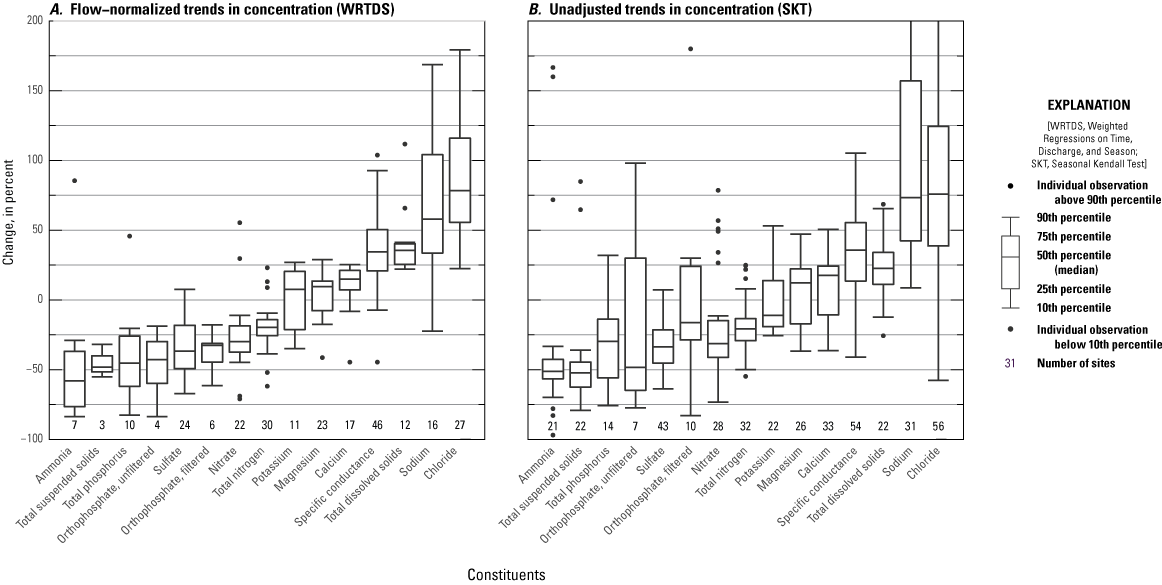
Percentage change in concentration of significant trends for each constituent, for A, flow−normalized trends in concentration calculated with Weighted Regressions on Time, Discharge, and Season and B, unadjusted trends in concentration calculated with the Seasonal Kendall Test for the period of record trends. Percentage changes greater than 200 are not shown in this plot.
To understand patterns in changing water quality, it is necessary to interpret the percentage of sites with a significant trend direction and the magnitude of those significant trends. Although nutrient trends were generally decreasing rather than increasing or being nonsignificant, the percentage of sites with significant decreases in nutrient constituents tended to be less than the percentage of sites with significant increases in salinity constituents (fig. 5), although nutrient trend magnitudes can be comparable to those for TDS and SC (fig. 6). Sulfate, with the largest percentage of sites with decreasing trends, had median percentage changes less than −34 percent for both methods. Although ammonia and TSS had some of the largest magnitude decreases, most trends for these constituents were nonsignificant (figs. 5 and 6). Potassium was the only constituent with a positive median percentage change for one method (WRTDS) and negative for the other (SKT), but that is to be expected because, as noted above, the trend direction with the largest number of sites differed between methods. For potassium, both of the median percentage changes were small and the IQR of percentage changes straddled zero.
The trends assessed in this section are for the POR, which varies for each water-quality record. Thus, the length of time represented by each increasing, decreasing, and nonsignificant trend may be different, and the water-quality records assessed might represent different periods (although all periods end in 2017 or 2018). The POR trends were used here because the scope of this analysis is intended to be comprehensive and to capture all potential long-term changes in the water quality of the Delaware River Basin. We sought to summarize not just the most recent changes (2008–18 trend period), but to understand change as far back in time as it was possible at all sites. The results of these same analyses for identical periods, the 2008–18 trend period, are in the appendix (figs. 1.1 and 1.2), and the results for the 2008–18 trend period and the POR mostly agree.
Evolution of Changes in Water Quality
Assessing the rates of change for constituents with significantly decreasing or increasing trends can illustrate whether those changes are happening more quickly or slowly over time. The 5-year rates of change (milligram per liter per 5-year subperiod) for sulfate were all negative, and there were no positive rates at any site throughout the subperiods investigated, showing a very consistent decreasing trend direction for this constituent. Additionally, negative rates of change for sulfate decreased between 1998 and 2013, indicating faster decreases during this period, and those decreases continued, but at a slower rate after 2013 (fig. 7). The median rates of change for TP were negative for the subperiods spanning from 1993 to 2008, but the negative changes slowed down over time, with rates getting closer to zero, until the 2013–18 subperiod, during which the median rate of change shifted from negative to positive. This shift indicated that, by the 2013–18 subperiod, a larger number of sites had positive rates of change (increases in TP annual mean FN concentration), compared to negative rates of change (decreases in TP annual mean FN concentration). The pattern in negative rates of change (decreases) for TN and nitrate was similar for the subperiods investigated, which was to be expected because nitrate is often the majority component of TN. These parameters had decreasing median rates that largely leveled off to roughly a constant rate of decrease between 2003 and 2018 (fig. 7).
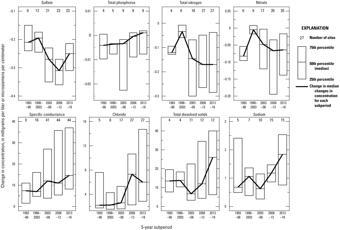
Interquartile ranges for rates of change in concentration between 5-year subperiods for all sites with significant Weighted Regressions on Time, Discharge, and Season trends for selected constituents, in the trend direction which contained the largest number of sites.
The constituents with primarily increasing trends (SC, chloride, TDS, and sodium) tended to display increasing rates of change over the 25 years investigated, indicating increases have been occurring at faster rates over this time. The median rates of change for TDS and sodium, in particular, showed noticeable increases between 2003 and 2018, whereas SC increases were steady, but more subtle, and chloride median rates were more variable in this period. The IQRs of the rates of change for the constituents with increasing trends tended to be wide in the more recent subperiods, for example, 2013–18, indicating higher variation in the rate of increases for these years, and potential rates of change much higher than the median, perhaps possible to assess because there were a greater number of sites in these years (fig. 7). For each of the eight constituents, however, wide IQRs were present for many subperiods, demonstrating considerable variation in rates of change between sites, although some general tendencies across sites did exist.
Level of Concern Comparisons
Figure 8 shows the results of categorizing the POR trends relative to the LOC for both trend methods. POR start- and end-year concentrations for sulfate, nitrate, ammonia, and chloride were all below the LOC, with the exception of one site with an SKT trend for nitrate, for which start- and end-year concentrations were above the LOC (fig. 8). Sulfate, nitrate, and ammonia trends were largely decreasing away from the LOC or were nonsignificant. Most of the chloride trends were increasing towards the LOC. Both methods had sites with TDS trends (3 sites with WRTDS trends and 1 site with an SKT trend) that increased above the LOC over the POR, representing an environmentally relevant degradation in water quality (fig. 8). Three of these sites were on the same tributary to the Delaware River, and all were in Pennsylvania. The WRTDS results showed 77 percent of chloride trends and 38 percent of TDS trends increasing towards the LOC. Similar percentages were apparent for SKT results with 66 percent of chloride trends and 47 percent of TDS trends also increasing towards the LOC, ultimately representing a potential threat to water quality.
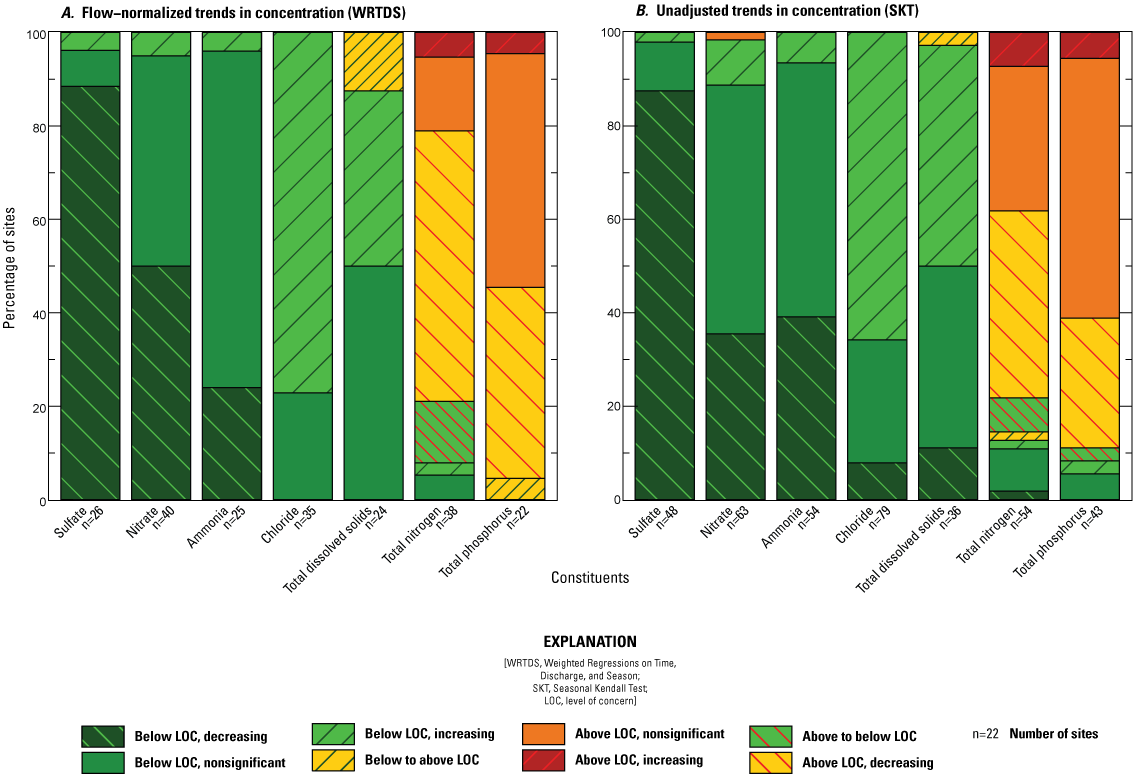
Percentage of sites for each constituent and trend method in the eight trend categories relative to the level of concern. Period of record trends were categorized by the relation of the start and end concentrations to the level of concern and trend direction.
Start and end concentrations for TN and TP trends were above the LOC at most sites, but between 28 percent and 58 percent of sites were trending downward toward the LOC (specifically, 58 percent of trends determined with WRTDS and 40 percent determined with SKT for TN and 41 percent of WRTDS trends and 28 percent of SKT trends for TP), indicating the potential for continued improvements in water quality at those sites (fig. 8). Trends in TN and TP produced the highest percentage of sites that crossed the LOC threshold, both from above and below the LOC. For TN, five sites (13 percent) with WRTDS trends and four sites (7 percent) with SKT trends decreased from above to below the LOC during the POR, demonstrating improved water quality. For TP, only one site with an SKT trend decreased from above to below the LOC. Notable degradations in water quality were seen for one TP site with a WRTDS trend (Neversink River near Claryville, New York; fig. 1.18B) and one TN site with an SKT trend (Brodhead Creek near East Stroudsburg, Pennsylvania; fig. 1.17A), which increased from below to above the LOC (fig. 8), although these particular trends were nonsignificant, indicating that the water-quality records used to determine the trends might have been highly variable or sparse.
Identifying environmentally important changes that occurred over the longest period possible (POR trends) helps to place long-term changes in context (fig. 8), but to assess current water-quality threats and successes, understanding more recent change is also necessary. The 2008–18 trends that were approaching an LOC from either above (improving) or below (degrading) were investigated to understand how close the trend end concentrations (2018) were to the LOC. Of the 105 trends that were increasing toward the LOC from below, only five sites (5 percent) had end concentrations within 60 percent of the LOC, with trends in chloride, TN, TP, and TDS (fig. 9). For the 37 site constituents that were decreasing towards the LOC from above, only 3 sites (8 percent) had end concentrations within 160 percent of the LOC, with trends in TN and TP (fig. 9). Overall, 94 percent of trends from both methods were greater than 160 percent of the LOC or less than 60 percent of the LOC. Thus, even though some constituents had many trends approaching the LOC, many of the sites had concentrations that were still much higher or lower than the LOC, indicating that between 2008 and 2018, immediate degradation or improvement was not likely for many of the water-quality sites and constituents.
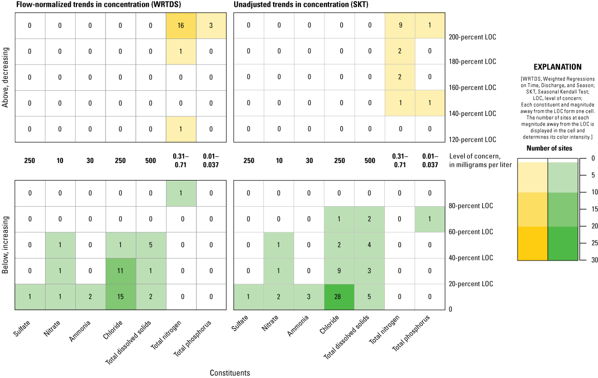
The number of sites with 2008–18 trend end concentrations at varying proximities to the level of concern (LOC), by constituent, for each trend method in the “below LOC, increasing” and “above LOC, decreasing” categories.
To understand how water quality might change in the future, the rate of change for the 2008–18 trends approaching the LOC in the “below LOC, increasing” and “above LOC, decreasing” categories was projected into the future to estimate the number of years to reach the LOC. For increasing trends in sulfate, nitrate, ammonia, chloride, and TDS that are approaching the LOC, the median number of years to reach the LOC was greater than 80 regardless of trend method, indicating that for most of these sites and constituents, the rates of change are small and there was no immediate threat of crossing the LOC (fig. 10). For chloride and TDS, however, notable outliers are observed, with the number of years to reach the LOC dropping as low as 12 for one site with a chloride SKT trend (Valley Creek at Wilson Road near Valley Forge, Pa.) (fig.10). Furthermore, the one TN trend (WRTDS result) and the one TP trend (SKT result) that were increasing towards the LOC had end concentrations near the LOC (fig. 9) and large enough rates of change to indicate only 2.5 and 11 years, respectively, to potentially reach the LOC (fig. 10).
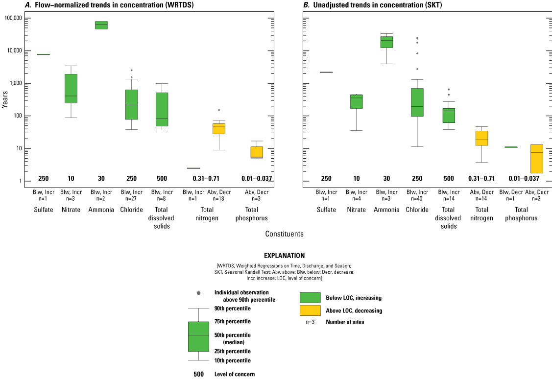
The distribution of the number of years for concentrations to equal the level of concern for each constituent for A, flow-normalized trends in concentration using Weighted Regressions on Time, Discharge, and Season and B, unadjusted trends in concentration using the Seasonal Kendall Test for the 2008–18 trends in the “below LOC, increasing” and “above LOC, decreasing” categories.
Alternately, for TN trends decreasing towards the LOC, the median number of years to reach the LOC was less than 50, and for TP trends decreasing towards the LOC, the median number of years to reach the LOC was less than 8, indicating that decreases in TN and TP concentrations at these sites might cause the ecoregional nutrient criteria to be met relatively soon (fig. 10). In summary, most of the 2008–18 TN and TP trends that were decreasing towards the LOC had faster rates of change compared to the trends increasing towards the LOC, producing a comparatively short timeframe to achieve water-quality improvement (fig. 10).
Land-Use Assessment and Land-Surface Change
Of the 124 unique sites used in this analysis, 9 changed land-use categories at some point during the POR. In all cases, these nine sites became more urbanized. As of 2017, most sites were mixed use (63), about half that many were undeveloped (32), 22 sites were urban, and only 7 sites were agricultural (table 4). When subdivided by trend method, the relative frequency of sites in land-use categories is similar (table 4). Because of the small number of agricultural sites, water-quality trends at these sites will not be discussed.
Table 4.
Land-use categorization of sites for 2017.[Sites with Weighted Regressions on Time, Discharge, and Season results and sites with Seasonal Kendall Test results do not add to all unique sites because sites often have trends for multiple constituents, some of which may have Weighted Regressions on Time, Discharge, and Season results and others Seasonal Kendall Test results. WRTDS, Weighted Regressions on Time, Discharge, and Season; %, percent; n, number; SKT, Seasonal Kendall Test]
Across all constituents, undeveloped sites tended to have water-quality trends that were lower in magnitude and had less variability between sites compared to mixed-use and urban sites (fig. 11). For SC, TDS, and most major ions, mixed-use and urban sites consistently had increasing trends, and urban sites had some of the largest increases, except for sulfate trends which decreased over the POR for sites in all land-use categories. For nutrients and TSS, mixed-use and urban sites tend to be decreasing but less consistently than the increases seen for the salinity constituents and most of the major ions (fig. 11). For percentage change, trends at undeveloped sites have relative magnitudes of change more similar to mixed-used sites (fig. 12). This is particularly evident for constituents such as TN, nitrate, TSS, SC, TDS, chloride, and sodium, indicating small magnitude changes in concentration observed at undeveloped sites are sizable compared to their starting concentrations (fig. 12).
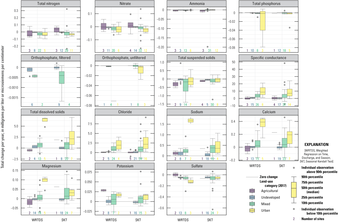
Total change in concentration per year over the length of the period of record trend, in milligrams per liter or microsiemens per centimenter, per year, by constituent, trend method, and 2017 land-use categorization.
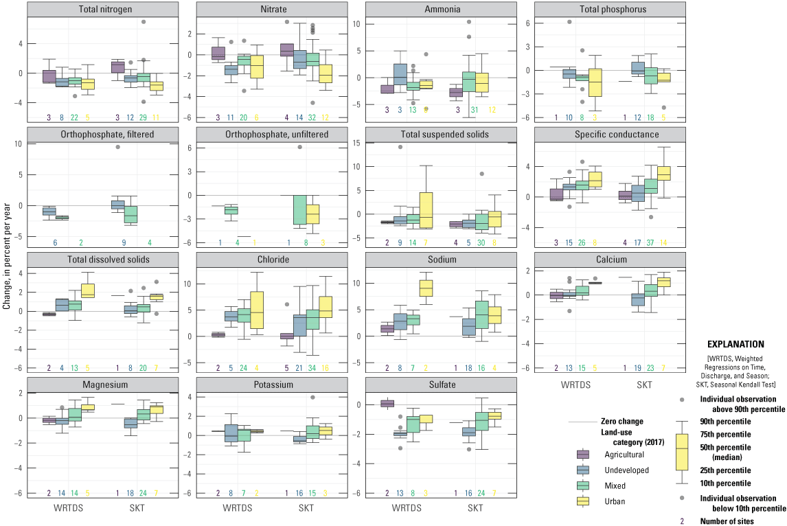
Percentage change in concentration per year over the length of the period of record trend, by constituent, trend method, and 2017 land-use categorization. Four Seasonal Kendall Test trends greater than 40 percent change are not shown.
Across all sites, cumulative land-surface change ranged from 0 to 49 percent, with a median of 10 percent, indicating that at half of the sites at least 10 percent of a given watershed had land-surface changes over the POR (fig. 13). This metric captures a range of land-surface changes, from permanent changes such as the expansion of suburban development, to transient changes such as the destruction of vegetation and infrastructure due to severe weather. The metric also captures multiple changes to the same spatial area over the POR, and it includes changes that may not cause a watershed to change land-use categorizations. Determining specifically what land-surface changes occurred in the watersheds included in this report would require an indepth look at additional land-surface imagery over time, a task not completed as a part of this analysis. Unsurprisingly, urban sites had the largest cumulative changes, followed by mixed-use and agricultural sites; undeveloped sites mostly had cumulative land-surface changes less than 5 percent over the POR (fig. 13). When plotted against the concurrent water-quality POR trend, cumulative land-surface change had a strong positive relation with all salinity-related constituents and major ions, except sulfate (fig. 14), indicating sites with more land-surface changes in the watershed also had larger increases in concentration for these constituents. For sulfate, decreases were consistent across all magnitudes of cumulative land-surface change, showing no relation between land-surface change and change in sulfate concentration. Similarly, TN and nitrate trends were unrelated to cumulative land-surface change. While TP and TSS showed no relation between land-surface change and the SKT trend, the WRTDS trend results showed negative relations with some scatter for these constituents (fig. 14). The plots of water-quality change versus cumulative percentage of land-surface change for the 2008–18 period are in the appendix (fig. 1.4).
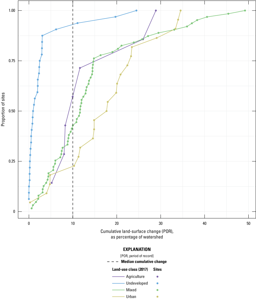
Empirical cumulative distribution function of the cumulative land surface that changed over the longest period of record at each site, as a percentage of the watershed, grouped by land-use classification in 2017. Of the 124 unique sites, 11 sites had water-quality records that are longer than the Land Change Monitoring, Assessment, and Projection data used to generate the cumulative land-surface change metrics.
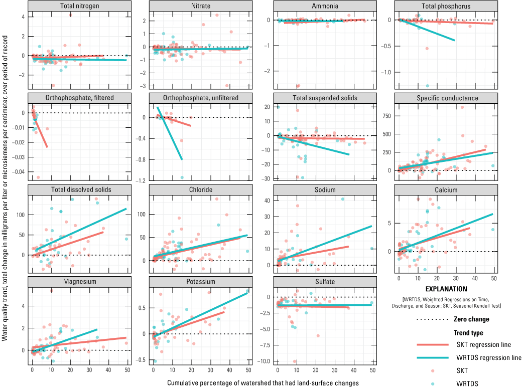
Total change in water-quality for the period of record versus the cumulative change in land-surface cover over the same period, as a percentage of the watershed, by trend method type.
Spatial Summary
Strong relations between geographic location and trend direction or magnitude were not observed in the POR trends for most constituents (figs. 1.5–1.19). Calcium, nitrate, orthophosphate (filtered and unfiltered), TDS, TN, and TP had no spatial patterns, or weak patterns. Chloride had large magnitude increases throughout the basin (fig. 1.7), and likewise, sodium and SC were increasing consistently basinwide (figs. 1.14 and 1.13). Significant SKT trends for ammonia were clustered in the southern part of the basin and were mostly decreases (fig. 1.5). Where there were significant trends for magnesium and potassium, the decreases tended to occur in the upper basin and increases in the lower basin, although the magnitude of these changes was small (figs. 1.8 and 1.12). Decreasing TSS trends estimated with SKT are evident in the southern part of the basin (fig. 1.19), whereas the largest decreases in sulfate tend to occur in the northern part of the Delaware River Basin (fig. 1.15). The POR trends do not represent the same period for each constituent and site, however, so this might make spatial patterns more difficult to detect.
Comparison of WRTDS and SKT Trends
As discussed above, for some sites, constituents, and trend periods, the criteria for both SKT and WRTDS were met, and trend results were generated with both methods. For the 993 results in which trend direction was available for both methods, 75 percent of the results agreed, generating significant trends in the same direction or nonsignificant trends with both methods (table 5). The other 25 percent of results produced significant trends with one method, but nonsignificant trends with the other (table 5). The methods produced significant trends in conflicting directions only once. The number of results in each trend direction comparison group, for each constituent, are in the appendix (table 1.2). In addition to the general agreement of trend direction between methods, when the two methods produced significant trends in the same direction, they also tended to result in a comparable percentage change. For the pairs of results in which the methods agreed on significance and trend direction, 70.4 percent of the pairs had a difference in percentage change that was less than 10, and an additional 18.6 percent of the pairs had differences in percentage change greater than 10 but less than 20 (table 6). The absolute differences in percentage change by constituent are in the appendix (tables 1.3). Note that due to data censoring, sometimes a tau value but not a sen slope was reported for SKT results (as discussed in the “Trend Estimation” section). Therefore, because SKT sometimes allows for the calculation of trend direction, but not percentage change, the number of results with significant trend direction agreement does not match the number of results that can be assessed for trend magnitude agreement.
Table 5.
Number of trend results determined by Weighted Regressions on Time, Discharge, and Season and Seasonal Kendall Test methods in each trend direction comparison group.[SKT, Seasonal Kendall Test; WRTDS, Weighted Regressions on Time, Discharge, and Season]
Table 6.
Absolute difference in percentage change between trend result pairs determined by Weighted Regressions on Time and Season and Seasonal Kendall Test methods when the trend direction was significant and in agreement.[x, absolute difference in percentage change; <, less than; >, greater than]
Discussion
This report summarizes changes in surface-water quality in the Delaware River Basin for salinity, major ions, nutrients, and suspended solids using multisource data and two trend methods. Water quality affects the suitability of water for human and ecological uses. Understanding how water quality has changed in relation to levels of concern, land-use/surface changes, and spatial extent can indicate potential threats to water availability. Similarly, this understanding can help identify areas of progress and track the success of efforts to improve, maintain, and protect water for various uses. In this section, we summarize the results of our analysis by constituent group and present key findings, areas for improved assessment, and data gaps.
Salinity and Major Ions
Chloride and SC were ranked among the top four constituents with the largest number of sites with water-quality data for both methods, indicating that they are among the best represented constituents in this analysis (table 3). Figure 7 showed generally increasing rates of change for these constituents, indicating that increasing trends are occurring at faster rates over time. Chloride, for example, had increasing trends with changes as high as 200 percent and rates of change increasing by more than 15 milligrams per liter per 5-year subperiod at some sites. Annual mean chloride concentrations, however, were still greatly below the 250 mg/L LOC (a secondary drinking water standard) at all sites, and the median number of years to reach the LOC was predicted to be greater than 100. In contrast, TDS showed the greatest cause for concern in the LOC analysis because concentrations at four sites increased above the LOC (also a secondary drinking water standard) during the POR, a notable percentage of sites (43 percent) were increasing towards the LOC, and two sites had trend-end concentrations (2018) relatively near the LOC (within 40 percent of the LOC). Calcium, magnesium, and potassium are represented in this analysis with 36 to 50 SKT trends and 19 to 35 WRTDS trends, depending on the constituent. These major ions have relatively even proportions of increasing, decreasing, and nonsignificant trends (fig. 5), and their changes are generally +/−25 percent and distributed around zero (fig. 6), indicating that water-quality changes in these constituents are small, variable between sites, and not of great concern basinwide. The greatest total changes per year and percentage changes per year for the salinity constituents, chloride, sodium, calcium, and magnesium occurred mostly at sites with urban land use, although sites with mixed and undeveloped land use were occasionally at comparable levels. Cumulative land-surface change had a strong positive relation with water-quality change for the salinity constituents, chloride, sodium, calcium, and potassium, indicating that changes on the land surface may be one of the factors contributing to widespread increases in salinity and these major ions. Increasing trends in SC, chloride, and sodium were basinwide, illustrating the widespread nature of this change.
Water availability for human health and aquatic life is threatened by increasing salinization that degrades the quality of freshwater. This degradation can threaten drinking water sources, which is of particular concern for the Delaware River Basin, which supplies drinking water to over 13 million people (Delaware River Basin Commission, 2020a). Assessing increases in chloride and the chloride-sulfate mass ratio are two ways that water-quality trends can be used to evaluate the potential for stream water to create corrosive conditions in drinking water infrastructure (Stets and others, 2018). Corrosion of water distribution systems can cause lead, copper, and other metals to leach into drinking water (Ng and Lin, 2016) and present a potential public health issue or the need for more costly drinking water treatment (Cañedo-Argüelles and others, 2016). The results presented in this report show widespread increases in surface-water chloride concentrations (fig. 5, fig. 1.7). Of the 21 sites with chloride and sulfate POR trends, 13 sites (62 percent) had increasing chloride trends and decreasing sulfate trends, indicating the potential for an increasing chloride-sulfate mass ratio.
Elevated salinity can also cause lethal and sublethal effects on aquatic communities (Hart and others, 1991). These effects are especially relevant in the Delaware River Basin, which supports a trout fishery and endangered fish and mussel species (Delaware River Basin Commission, 2020a). Water-quality degradation is a serious threat to these species, including the endangered Alasmidonta heterodon (dwarf wedgemussel) and other freshwater mussels, in the Delaware River Basin, which are sensitive to many contaminants, including chloride (U.S. Fish and Wildlife Service, 2011). Sodium chloride and calcium chloride have also been shown to have effects on the growth of trout species (Hintz and Relyea, 2017).
The salinity constituents (TDS and SC) had trend patterns similar to sodium and chloride, suggesting sodium and chloride were the source of overall salinity changes (that increases in TDS and SC may be caused by increases in chloride and sodium). A likely source of these major ions in the Delaware River Basin is sodium chloride deicing salt. Our finding the greatest change in SC, TDS, chloride, and sodium at sites with urban land use agrees with Stets and others (2018), who noted a high potential for increased corrosivity in urban areas. Additionally, the strong correlation between land-surface change and water-quality change for salinity and most major ions indicates that increasing urbanization and deicing salt application in urban areas might be a driver of these trends in the Delaware River Basin.
Previous studies in the Northeast United States, and the Delaware River Basin specifically, have noted similar increases in salinity-related constituents over time (Kaushal and others, 2005; Oelsner and others, 2017; Delaware River Basin Commission, 2019). This study found widespread increases in SC, TDS, chloride, and sodium, and found that increases in the salinity constituents and sodium are occurring more quickly in recent years. Continued salinization of rivers and streams in the Delaware River Basin at a quickening pace suggests the need for more urgent salinity management across the Delaware River Basin, including the need to definitively determine and mitigate the drivers of changes in salinity concentrations. Continued and additional monitoring of sodium in the western Delaware River Basin and TDS in the upper Delaware River Basin would provide information to fill the spatial gaps in this analysis. Calcium, magnesium, and potassium do not generally present water-quality concerns in the Delaware River Basin, although their continued study can advance the understanding of the drivers of salinity changes, ion exchange and mineral dissolution, and of groundwater/surface-water interactions, which can all affect water quality and have been noted as an area of interest in the Delaware River Basin (Fischer, 1999; USGS, 2020).
Alternately, sulfate trends have strong widespread decreases: more than 85 percent of sites for both trend methods show decreases (fig. 5) and exhibit some tendency to decrease at faster rates in recent years (fig. 7). The start and end concentrations of sulfate trends were below the LOC at all sites (fig. 8). At two sites, trends were increasing towards the LOC, but trend projections show greater than 2,000 years would be required to reach the LOC if the rate of change from 2008 to 2018 continued into the future (fig. 10). The decreases in sulfate concentrations seen in Delaware River Basin rivers and streams have been observed throughout the United States in response to decreases in the atmospheric deposition of sulfur related to the enactment of the Acid Rain Program, established under the Clean Air Act (EPA, 2020b). Instream changes in sulfate concentration and watershed land-surface changes were not related in our analysis (fig. 14), which suggests that atmospheric deposition was the primary driver of change. Despite general decreases of instream sulfate concentrations throughout the U.S., applications of sulfur to agricultural fields to assist in plant uptake of nitrogen have increased, in response to the reductions in atmospheric sulfate deposition and thus reductions in sulfate available for plant metabolism (Hinckley and others, 2020). There is record of sulfur application for these purposes in the Northeastern U.S., which has the potential to counteract decreasing trends, and might be the reason for the slowing rate of decrease for sulfate in the Delaware River Basin shown in figure 7 (Ketterings and others, 2012).
Nutrients
Several nutrient constituents (ammonia, nitrate, TN, and TP) are well represented in this analysis (42 to 63 SKT trends and 22 to 40 WRTDS trends), depending on the constituent. Orthophosphate and TN trends were among the constituents with the largest percentages of decreasing trends (fig. 5), but all nutrient constituents had negative median percentage changes (fig. 6), although these constituents can have a substantial percentage of sites with nonsignificant trends (fig. 5). Decreasing rates of change were observed for nitrate and TN, leveling out to a relatively constant rate of decrease in their instream concentrations by 2018 (fig. 7). A high percentage of trend-period start and end concentrations were above the LOC for TN and TP, although several sites had POR trends that decreased below the LOC, indicating meaningful water-quality improvement (fig. 8). If rates of change were to remain constant, every site with a TN trend decreasing towards the LOC would cross below the LOC threshold in less than 75 years, and this estimate would be 17 years for TP (fig. 10).
Nutrients threaten natural waters in many ways, including contributing to harmful algal bloom prevalence (which can cause serious human health consequences) and excessive algal growth (which upon senescence, can decrease dissolved oxygen concentrations critical for the health of fish and aquatic communities) (EPA, 2020a). In the Delaware River Basin, elevated concentrations of nitrogen have been identified as a potential cause of water-quality degradation in the Delaware Estuary (Delaware River Basin Commission, 2020b). In response to this threat, nutrient management initiatives addressing the main stem of the Delaware River and Estuary were established, and the recent status of nutrients in the Delaware River Basin has been reported as “very good” (Delaware River Basin Commission, 2019). Our analysis of long-term water-quality trends supports this assessment by showing generally decreasing concentrations, which indicates ongoing nutrient reduction strategies may be successful. Despite these general decreases, the LOC analysis showed that the majority of TN and TP concentrations in 2018 were greater than the EPA ecoregional nutrient criteria. These criteria represent a starting point for States to use in developing water-quality standards that protect freshwater systems from the effects of excess nutrient input (EPA, undated c). Exceedances of these criteria indicate that continued nutrient monitoring and management in the Delaware River Basin is warranted. In particular, orthophosphate monitoring is not well distributed spatially in the basin, and it was possible to estimate trends in orthophosphate at only a small number of sites, even with the less stringent SKT criteria.
Suspended Solids
As noted in the “Methods” section, only one site passed the criteria to generate a trend for suspended sediment concentration, so changes in sediment were represented in this analysis by TSS, for which 83 SKT and 32 WRTDS trends were calculated. TSS had the largest percentage of nonsignificant trends for all constituents with WRTDS trends (91 percent) and many nonsignificant SKT trends (59 percent) (fig. 5). When significant, TSS trends were decreasing with large negative percentage changes (fig. 6). Across both methods, only one TSS trend showed a significant increase over the POR. Nonsignificant trends occur for many reasons, such as generally stable water-quality concentrations over time, highly variable water-quality concentrations (noisy data), sparse data records given the variability of the data, and difficulty of the model to characterize the patterns of variability. Furthermore, sediment is notoriously difficult to model because most sediment is transported during high streamflows, which are typically less sampled than lower flows. Additionally, compared to suspended sediment concentration determinations, TSS determinations are less accurate, less precise, and are often biased low when there is a high fraction of suspended sand in the water column. TSS can poorly represent suspended sediment in natural waters (Gray and others, 2000): a potential explanation for the high proportion of nonsignificant trends for this constituent. However, an alternative explanation may be that TSS has been largely stable over the POR in the Delaware River Basin, and any small changes that may have occurred were not detected.
Understanding changing sediment in the Delaware River Basin is important for maintaining the health of surface waters in the basin, from the Delaware estuary to the upper most headwaters. The erosion of sediment from stream banks in the basin is a major source of new sedimentation in the estuary, and the Delaware Estuary Regional Sediment Management Plan notes the need to “fully characterize sediment processes and outputs” in the basin (Delaware Estuary Regional Sediment Management Plan Workgroup, 2013). Additionally, 90 percent of the water supply to New York City originates in the Catskill and Delaware watersheds, with the Cannonsville, Pepacton, and Neversink Reservoirs falling within the Delaware River Basin (Committee to Review the New York City Watershed Protection Program, 2020). These reservoirs are the largest unfiltered water supply source in the United States, and the maintenance of their water quality is critical in maintaining a potable water supply to the largest city in the United States. Therefore, understanding the trends and current conditions of turbidity is a top priority for the New York City Watershed Protection Program (Committee to Review the New York City Watershed Protection Program, 2020). Turbidity and TSS are strongly related, so the decreasing TSS trends in the Delaware River Basin are a positive result for watershed protection and potential sediment transport, indicating potential progress has been made in reducing sediment erosion in the Delaware River Basin. Furthermore, the large percentage of nonsignificant trends may also be a cautiously positive result, indicating that at many sites sediment concentrations may have changed very little and historical conditions have been maintained over time. Even in light of improving or maintained TSS conditions in many streams across the Delaware River Basin, continued data collection, especially at high flows, may allow for more robust trends to be generated in the future, and using suspended sediment concentration determinations in place of TSS may increase the accuracy and precision of the data and the ability to detect smaller changes over time.
Trend Method Strengths and Weaknesses
As described in the “Introduction” and “Methods” sections, the two trend methods used in this study have strengths and weaknesses to consider in the interpretation of their results. However, the analysis in the “Comparison of WRTDS and SKT trends” section indicates that, in terms of trend direction and magnitude, the methods produce mostly comparable results (tables 5 and 6). Across all combinations of site, constituent, and trend period used in the WRTDS-SKT comparison, 19 percent of the combinations had a significant trend detected using WRTDS but not using SKT, likely because controlling for streamflow allows WRTDS to identify a trend that may have been otherwise obscured due to variable weather and streamflow conditions. For the 6 percent of results in which SKT detected a significant trend in water quality, but WRTDS did not, it is likely these trends are due to several higher-than-average or lower-than-average flow years at the beginning or end of the trend period, causing an apparent trend in water quality. Because these apparent trends might be entirely due to variable streamflow (in other words, some years are wetter or drier than others), when flows return to more average conditions in coming years, they are likely to dissipate. The flow-normalization techniques used in WRTDS to characterize trends guard against these apparent, temporary trends by accounting for the interannual and often periodic variability of precipitation and streamflow, something SKT is incapable of capturing. Ultimately, conflicting trend directions occurred at only a single site, indicating the comparability of the results generated in this analysis. The magnitude of change is also important in assessing the status of water quality in a basin. Trend magnitudes estimated with WRTDS and SKT were largely consistent, with 89 percent of the compared results generating percentage changes that were within 20 percent of each other (table 6).
The WRTDS and SKT trend estimation techniques use distinctly different approaches for estimating trends, in particular, the inclusion of streamflow as a covariate with WRTDS. Despite these different approaches, the overall agreement of trend direction and magnitude in the Delaware River Basin indicates that SKT might be a suitable method to assess changing water quality when streamflow data is not available. Although WRTDS allows for a much more refined and certain understanding of changing water quality, analysts with limited data availability might be willing to use SKT trend estimation instead, considering the general agreement of results in the Delaware River Basin presented in this report. Tables 1.2 and 1.3 provide more information on the reliability of SKT results for specific constituents. The overall comparability of the trend results might indicate that streamflow does not substantially affect changes in water quality in the Delaware River Basin and that watershed management, such as changes in point and nonpoint sources, might be driving changing water quality.
Summary
This report, which assesses and summarizes changing water quality in the Delaware River Basin, identified constituents which present potential threats to water availability and also noted constituents for which efforts to improve surface-water quality have been successful. The increasing concentrations of the salinity constituents, chloride, and sodium and their mostly increasing rates of change are another line of evidence in the growing body of work finding the concentrations of these parameters to be a cause for concern in the Delaware River Basin and the Northeastern United States. In particular, increases in the concentrations of these constituents, along with the decreasing trends in sulfate, present the potential for increased corrosivity of drinking water infrastructure. The decreasing nutrient concentrations at some sites in this report, the shifts of total nitrogen and total phosphorus at some sites from above to below the level of concern (EPA ecoregional nutrient criteria), and the rates of change that indicate a relatively short timeframe for total nitrogen and total phosporus concentrations to fall below the level of concern support recent assessments completed by other organizations that also identify improving water quality due to the efficacy of nutrient-focused water-quality protection programs. The total nitrogen and total phosphorus concentrations at most sites are still above the level of concern, however, illustrating the need for the continuation of these programs. The concentrations and trends of suspended solids, calcium, magnesium, and potassium identified in this study do not warrant immediate concern, although continued data collection and assessment may improve the ability to identify changes, or lack thereof, in these constituents, many of which had nonsignificant trends in this study. The maintenance and protection of water for human health and ecosystems is a global priority, and in the Delaware River Basin where people rely on safe drinking water, healthy ecological communities that support endangered species, clean water for crop irrigation, and low corrosivity water for industrial processes, understanding water-quality trends and current conditions can help water managers protect this valuable resource.
Acknowledgments
The authors gratefully acknowledge Danielle Folette and Mary Kate Perkins of the U.S. Geological Survey for their assistance in the Weighted Regressions on Time, Discharge, and Season model review and Meghan Hian and Emily Gain of the U.S. Geological Survey for their work creating maps.
References Cited
Brown, J.F., Tollerud, H.J., Barber, C.P., Zhou, Q., Dwyer, J.L., Vogelmann, J.E., Loveland, T.R., Woodcock, C.E., Stehman, S.V., Zhu, Z., Pengra, B.W., Smith, K., Horton, J.A., Xian, G., Auch, R.F., Sohl, T.L., Sayler, K.L., Gallant, A.L., Zelenak, D., Reker, R.R., and Rover, J., 2020, Lessons learned implementing an operational continuous United States national land change monitoring capability—The land change monitoring, assessment, and projection (LCMAP) approach: Remote Sensing of Environment, v. 238. [Also available at https://doi.org/10.1016/j.rse.2019.111356]
Cañedo-Argüelles, M., Hawkins, C.P., Kefford, B.J., Schäfer, R.B., Dyack, B.J., Brucet, S., Buchwalter, D., Dunlop, J., Frör, O., Lazorchak, J., Coring, E., Fernandez, H.R., Goodfellow, W., González Achem, A.L., Hatfield-Dodds, S., Karimov, B.K., Mensah, P., Olson, J.R., Piscart, C., Prat, N., Ponsá, S., Schulz, C.-J., and Timpano, A.J., 2016, Saving freshwater from salts: Science, v. 351, no. 6276, p. 914–916. [Also available at https://doi.org/10.1126/science.aad3488.]
Choquette, A.F., Hirsch, R.M., Murphy, J.C., Johnson, L.T., and Confesor, R.B., 2019, Tracking changes in nutrient delivery to western Lake Erie—Approaches to compensate for variability and trends in streamflow: Journal of Great Lakes Research, v. 45, no. 1, p. 21–39. [Also available at https://doi.org/10.1016/j.jglr.2018.11.012.]
Committee to Review the New York City Watershed Protection Program, 2020, Review of the New York City Watershed Protection Program: Washington, D.C., The National Academies Press, 418 p., accessed November 18, 2020, at https://www.nap.edu/read/25851/.
De Cicco, L.A., Hirsch, R.M., Lorenz, D., Watkins, W.D., 2018, dataRetrieval—R packages for discovering and retrieving water data available from Federal Hydrologic web services, accessed July 19, 2022, at https://doi.org/10.5066/P9X4L3GE.
Delaware Estuary Regional Sediment Management Plan Workgroup, 2013, Delaware Estuary Regional Sediment Management plan: [variously paged], 7 app., accessed June 30, 2021, at https://www.state.nj.us/drbc/library/documents/RSMPaug2013final-report.pdf.
Delaware River Basin Commission, 2016, Assessment of measurable changes to existing water quality, Round 1—Baseline EWQ (2000-2004) vs. Post-EWQ (2009-2011): 22 p., 3 app., accessed July 19, 2022 at https://www.nj.gov/drbc/programs/quality/lower-delaware_EWQassessment2016.html.
Delaware River Basin Commission, 2018, Special protection waters—Keeping the clean water clean: Deleware River Basin Commission Fact Sheet, 1 p., accessed July 19, 2022, at https://www.nj.gov/drbc/library/documents/SPW.pdf.
Delaware River Basin Commission, 2019, State of the Basin 2019: Delaware River Basin Commission State of the Basin Report, 55 p., accessed July 19, 2022, at https://www.state.nj.us/drbc/library/documents/SOTBreport_july2019.pdf.
Delaware River Basin Commission, 2020a, Basin information: Deleware River Basin Commission web page, accessed November 18, 2020, at https://www.state.nj.us/drbc/basin/.
Delaware River Basin Commission, 2020b, Dissolved oxygen and nutrients: Delaware River Basin Commission web page, accessed November 18, 2020, at https://www.state.nj.us/drbc/programs/quality/DO_nutrients.html.
Fischer, J.M., 1999, National Water-Quality Assessment Program—Delaware River Basin: U.S. Geological Survey Fact Sheet 1999–0056, 6 p., accessed November 18, 2020, at https://pubs.usgs.gov/fs/1999/0056/report.pdf.
Gray, J.R., Glysson, G.D., Turcios, L.M., and Schwarz, G.E., 2000, Comparability of suspended-sediment concentration and total suspended solids data: U.S. Geological Survey, Water-Resources Investigations Report 2000–4191, 14 p. [Also available at https://doi.org/10.3133/wri004191.]
Hart, B.T., Bailey, P., Edwards, R., Hortle, K., James, K., McMahon, A., Meredith, C., and Swadling, K., 1991, A review of the salt sensitivity of the Australian freshwater biota: Hydrobiologia, v. 210, 105–144 p. [Also available at https://doi.org/10.1007/BF00014327.]
Helsel, D.R., Hirsch, R.M., Ryberg, K.R., Archfield, S.A., and Gilroy, E.J., 2020, Statistical methods in water resources: U.S. Geological Survey Techniques and Methods, book 4, chapter A3, 458 p. [Also available at https://doi.org/10.3133/tm4A3.] [Supersedes U.S. Geological Survey Techniques of Water-Resources Investigations, book 4, chap. A3, version 1.1.]
Hinckley, E.L.S., Crawford, J.T., Fakhraei, H., and Driscoll, C.T., 2020, A shift in sulfur-cycle manipulation from atmospheric emissions to agricultural additions: Nature Geoscience, v. 13, p. 597–604. [Also available at https://doi.org/10.1038/s41561-020-0620-3.]
Hintz, W.D., and Relyea, R.A., 2017, Impacts of road deicing salts on the early-life growth and development of a stream salmonid—Salt type matters: Environmental Pollution, v. 223, p. 409–415. [Also available at https://doi.org/10.1016/j.envpol.2017.01.040.]
Hirsch, R.M., Archfield, S.A., and De Cicco, L.A., 2015, A bootstrap method for estimating uncertainty of water quality trends: Environmental Modelling & Software, v. 73, p. 148–166. [Also available at https://doi.org/10.1016/j.envsoft.2015.07.017.]
Hirsch, R.M., De Cicco, L.A., 2015, User guide to exploration and graphics for RivEr Trends (EGRET) and dataRetrieval—R packages for hydrologic data (ver. 2.0, February 2015): U.S. Geological Survey Techniques and Methods book. 4, 93 p., 2 app. [Also available at https://doi.org/10.3133/tm4A10.]
Hirsch, R.M., and De Cicco, L.A., 2018, Guide to EGRETci 2.0 enhancements: EGRETci web page, accessed May 8, 2020, at http://usgs-r.github.io/EGRETci/articles/Enhancements.html.
Hirsch, R., De Cicco, L., and Murphy, J., 2018a, EGRETci—Exploration and graphics for RivEr trends (EGRET) confidence intervals, version 2.0: EGRETci web page, accessed July 2022, at https://CRAN.R-project.org/package=EGRETci.
Hirsch, R., De Cicco, L., Watkins, D., Carr, L., and Murphy, J., 2018b, EGRET—Exploration and graphics for RivEr trends, version 3.0, accessed July 2022, at https://CRAN.R-project.org/package=EGRET.
Hirsch, R.M., Moyer, D.L., and Archfield, S.A., 2010, Weighted regressions on time, discharge, and season (WRTDS), with an application to Chesapeake Bay River inputs: Journal of the American Water Resources Association, v. 46, p. 857–880. [Also available at https://doi.org/10.1111/j.1752-1688.2010.00482.x.]
Hirsch, R.M., Slack, J.R., and Smith, R.A., 1982, Techniques of trend analysis for monthly water quality data: Water Resources Research, v. 18, no. 1, p. 107–121. [Also available at https://doi.org/10.1029/WR018i001p00107.]
Kaushal, S.S., Groffman, P.M., Likens, G.E., Belt, K.T., Stack, W.P., Kelly, V.R., Band, L.E., and Fisher, G.T., 2005, Increased salinization of fresh water in the northeastern United States: Proceedings of the National Academy of Sciences of the United States of America, v. 102. [Also available at https://doi.org/10.1073/pnas.0506414102.]
Ketterings, Q.M., Godwin, G., Gami, S., Dietzel, K., Lawrence, J., Barney, P., Kilcer, T., Stanyard, M., Albers, C., Cherney, J.H., Cherney, D., and Czymmek, K.J., 2012, Soil and tissue testing for sulfur management of alfalfa in New York State: Soil Science Society of America Journal, v. 76, p. 298–306. [Also available at https://doi.org/10.2136/sssaj2010.0437.]
Kummer, F., 2020, Delaware River named river of the year by national environmental organization: The Philadelphia Inquirer, April 15, 2020, accessed October 27, 2020, at https://www.inquirer.com/news/delaware-river-american-rivers-environment-20200415.html#:~:text=American%20Rivers%2C%20an%20environmental%20advocacy,by %20industrial%20and%20sewage%20waste.
Lorenz, D.L., [undated], smwrQW—An R package for managing and analyzing water-quality data, Version 0.7.9, accessed July 2022, at https://github.com/USGS-R/smwrQW.
Lorenz, D.L., 2015, smwrBase—An R package for managing hydrologic data (ver. 1.1.1): U.S. Geological Survey Open-File Report 2015–1202, 7 p., https://doi.org/10.3133/ofr20151202. [Superceded by Open-File Report 2016-1188, ver. 1.1.2].
Martin, G., Smoot, J., and White, K., 1992, A comparison of surface-grab and cross sectionally integrated stream-water-quality sampling methods: Water Environment Research, v. 64, p. 866–876. [Also available at https://doi.org/10.2175/WER.64.7.4.]
McKay, L., Bondelid, T., Dewald, T., Johnston, C., Moore, R., and Rea, A., 2012, NHDPlus version 2—User guide, 2012. U.S. Environmental Protection Agency, 183 p. [Also available at http://www.horizon-systems.com/NHDPlus/index.php.]
Murphy, J.C., and Sprague, L.A., 2019, Water-quality trends in US rivers—Exploring effects from streamflow trends and changes in watershed management: Science of the Total Environment, v. 656, p. 645–658. [Also available at https://doi.org/10.1016/j.scitotenv.2018.11.255.]
Murphy, J.C., Shoda, M.E. and Follette, D.D., 2020, Water-quality trends for rivers and streams in the Delaware River Basin using Weighted Regressions on Time, Discharge, and Season (WRTDS) models, Seasonal Kendall Trend (SKT) tests, and multisource data, water years 1978–2018: U.S. Geological Survey data release, https://doi.org/10.5066/P9KMWNJ5.
Murphy, J.C., and Shoda, M.E., 2020, Pooling resources across organizations—Multisource water-quality data for the Delaware River Basin: U.S. Geological Survey Fact Sheet 2020–3006, 2 p., https://doi.org/10.3133/fs20203006.
National Water Quality Monitoring Council, 2019, Water quality portal: National Water Quality Monitoring Council web page, accessed February 2019 at https://www.waterqualitydata.us/.
Ng, D.-Q., and Lin, Y.-P., 2016, Effects of pH value, chloride and sulfate concentrations on galvanic corrosion between lead and copper in drinking water: Environmental Chemistry, v. 13, no. 4, p. 602–610. [Also available at https://doi.org/10.1071/EN15156.]
Oelsner, G.P., Sprague, L.A., Murphy, J.C., Zuellig, R.E., Johnson, H.M., Ryberg, K.R., Falcone, J.A., Stets, E.G., Vecchia, A.V., Riskin, M.L., De Cicco, L.A., Mills, T.J., and Farmer, W.H., 2017, Water-quality trends in the Nation’s rivers and streams, 1972–2012—Data preparation, statistical methods, and trend results: U.S. Geological Survey Scientific Investigations Report 2017–5006, 136 p., https://doi.org/10.3133/sir20175006.
R Core Team, 2020, R—A language and environment for statistical computing: R Foundation for Statistical Computing, Vienna, Austria, https://www.R-project.org/.
Shoda, M.E., Murphy, J.C., Falcone, J.A., and Duris, J.W., 2019a, Multisource surface-water-quality data and U.S. Geological Survey streamgage match for the Delaware River Basin: U.S. Geological Survey data release, https://doi.org/10.5066/P9PX8LZO.
Shoda, M.E., Sprague, L.A., Murphy, J.C., and Riskin, M.L., 2019b, Water-quality trends in U.S. rivers, 2002 to 2012—Relations to levels of concern: Science of the Total Environment, v. 650, p. 2314–2324. [Also available at https://doi.org/10.1016/j.scitotenv.2018.09.377.]
Stets, E.G., Lee, C.J., Lytle, D.A., and Schock, M.R., 2018, Increasing chloride in rivers of the conterminous U.S. and linkages to potential corrosivity and lead action level exceedances in drinking water: Science of the Total Environment, v. 613–614, p. 1498–1509. [Also available at https://doi.org/10.1016/j.scitotenv.2017.07.119.]
Stone, W.W., Gilliom, R.J., and Martin, J.D., 2014, An overview comparing results from two decades of monitoring for pesticides in the Nation’s streams and rivers, 1992–2001 and 2002–2011: U.S. Geological Survey Scientific Investigations Report 2014–5154, 23 p. [Also available at https://doi.org/10.3133/sir20145154.]
U.S. Environmental Protection Agency, [EPA], 2018, 2018 Edition of the drinking water standards and health advisories tables: EPA Publication No. EPA 822-F-18-001, 20 p., accessed July 2022, at https://www.epa.gov/system/files/documents/2022-01/dwtable2018.pdf.
U.S. Environmental Protection Agency, [EPA], 2020a, Nutrient pollution: U.S. Environmental Protection Agency web page, accessed October 1, 2020, at https://www.epa.gov/nutrientpollution.
U.S. Environmental Protection Agency, [EPA], 2020b, Acid rain program: U.S. Environmental Protection Agency web page, accessed November 18, 2020, at https://www.epa.gov/acidrain/acid-rain-program.
U.S. Environmental Protection Agency, [EPA], [undated a], National primary drinking water regulations: U.S. Environmental Protection Agency web page, accessed October 1, 2020, at https://www.epa.gov/ground-water-and-drinking-water/national-primary-drinking-water-regulations.
U.S. Environmental Protection Agency, [EPA], [undated b], Secondary drinking water standards: Guidance for nuisance chemicals: accessed July 20, 2022, at https://www.epa.gov/sdwa/secondary-drinking-water-standards-guidance-nuisance-chemicals.
U.S. Environmental Protection Agency, [EPA], [undated c], Ecoregional nutrient criteria for rivers & streams documents: accessed July 20, 2022, at https://www.epa.gov/nutrient-policy-data/ecoregional-nutrient-criteria-rivers-and-streams.
U.S. Fish and Wildlife Service, 2011, Dwarf wedgemussel, U.S. Fish and Wildlife Service Fact Sheet, accessed July 13, 2021, at https://fws.gov/media/usfws-dwarf-wedgemussel-fact-sheet.
U.S. Geological Survey [USGS], 2019, USGS water data for the Nation: U.S. Geological Survey National Water Information System database, accessed July, 2019, at https://doi.org/10.5066/F7P55KJN.
U.S. Geological Survey, [USGS], 2020, Next generation water observing system—Delaware River Basin: U.S. Geological Survey web page, accessed November 18, 2020, at https://www.usgs.gov/mission-areas/water-resources/science/next-generation-water-observing-system-delaware-river-basin.
U.S. Geological Survey [USGS], [undated a], Advanced research computing, USGS Yeti Supercomputer: U.S. Geological Survey web page, [Also available at https://doi.org/10.5066/F7D798MJ.]
U.S. Geological Survey, [USGS], [undated b], Tracking water quality in U.S. streams and rivers, U.S. Geological Survey web page, accessed June 2021 at https://nrtwq.usgs.gov/nwqn/.
Wickham, H., François, R., Henry, L., and Müller, K., 2020, dplyr—A grammar of data manipulation, R package version 0.8.4, accessed July 2022 at https://CRAN.R-project.org/package=dplyr.
Wickham, H., and Henry, L., 2020, tidyr—Tidy messy data, R package version 1.0.2, accessed July 2022 at https://CRAN.R-project.org/package=tidyr.
Zhu, Z., and Woodcock, C.E., 2014, Continuous change detection and classification of land cover using all available Landsat data: Remote Sensing of Environment, v. 144, p. 152–171. [Also available at https://doi.org/10.1016/j.rse.2014.01.011.]
References Cited
Medalie, L., and Bexfield, L.M., 2020, Quality of data from the U.S. Geological Survey National Water Quality Network for water years 2013–17: U.S. Geological Survey Scientific Investigations Report 2020–5116, 21 p. [Also available at https://doi.org/10.3133/sir20205116].
Murphy, J.C., Shoda, M.E. and Follette, D.D., 2020, Water-quality trends for rivers and streams in the Delaware River Basin using Weighted Regressions on Time, Discharge, and Season (WRTDS) models, Seasonal Kendall Trend (SKT) tests, and multisource data, Water Year 1978-2018: U.S. Geological Survey data release [Also available at https://doi.org/10.5066/P9KMWNJ5.]
Oelsner, G.P., Sprague, L.A., Murphy, J.C., Zuellig, R.E., Johnson, H.M., Ryberg, K.R., Falcone, J.A., Stets, E.G., Vecchia, A.V., Riskin, M.L., De Cicco, L.A., Mills, T.J., and Farmer, W.H., 2017, Water-quality trends in the Nation’s rivers and streams, 1972–2012—Data preparation, statistical methods, and trend results: U.S. Geological Survey Scientific Investigations Report 2017–5006, 136 p. [Also available at https://doi.org/10.3133/sir20175006.]
Appendix 1. Supplemental Information
Additional Details on Data Processing
This section provides additional information about the water-quality data processing that was performed before trends analysis. The data processing steps described in the “Methods” section “Selection of Water-Quality Constituents and Additional Data Processing” and the following steps were performed to prepare the water-quality data for site clustering. This processing fits into the “selection of constituents and additional processing” step of the workflow illustrated in figure 1.
Data Combination
As discussed in the main text, for some constituents, data for multiple fractions were able to be reasonably combined for the estimation of a trend. For nitrate and nitrate+nitrite, data for multiple constituents were able to be reasonably combined and considered the same constituent. Table 1.1 outlines the combination of constituents and fractions in this study, based on the analysis of Oelsner and others (2017). Units were required to be unambiguous for data to qualify for combination, in other words, in the harmonized dataset (Shoda and others, 2019a), “flag_unitsAmbiguous” must equal “N” (please see Shoda and others, 2019a for more information, including a description of “flag_unitsAmbiguous”).
Table 1.1.
Constituent names used in this study, and the constituent and fraction that they correspond to in the harmonized dataset.[Some results were combined in this study and referred to with the same name. The ranking provided applied to results when data thinning was required due to multiple results for the same constituent at the same site and date. Harmonized dataset is from Shoda and others (2019a).+, plus; ---, constituents in which ranking was not needed; sum cnstnts, sum of constituents]
Result Removal
After results were combined for the constituents and fractions listed in table 1.1, some results were removed from the dataset:
-
• results with “>” remark codes;
-
• extreme outliers (results that exceed the mean of the logarithm of concentrations at a site by four standard deviations);
-
• results that included a summary statistic in the constituent name (for example, “Specific conductance, min”);
-
• results for suspended sediment concentration and total suspended solids that include the percentage of the sample with particle sizes (for example, “Suspended sediment concentration, pct <0.125mm”); and
-
• concentrations determined in the field for nutrient, major ion, salinity, and sediment constituents.
In the cases bulleted above, the result provided was ambiguous, likely in error, not representative of an in-stream water-quality concentration, or otherwise associated with increased uncertainty in the result value.
Data Thinning
In addition to the result removal noted in the section above, the dataset was “thinned” so that there was only one result per constituent, per site and day. Sometimes the combination of constituents and fractions at the same site created multiple results on the same day. Sometimes these multiple results occurred before data combination. When duplicate results were available for the same constituent and day at a site, the result that was used in trend estimation was chosen preferentially based on most desired constituent and fraction, as determined by Oelsner and others (2017) and listed in table 1.1. When a ranking of constituent and fraction was not available in Oelsner and others (2017), the result retained in the dataset was the constituent and fraction with the largest number of samples at that site. Any remaining duplication (multiple results for the same constituent at the same site and date) was resolved by randomly removing duplicates and retaining one result.
Data Adjustment
Lastly, Oelsner and others (2017) describes adjustments made to U.S. Geological Survey (USGS) data based on historical memorandums and reports. Medalie and Bexfield (2020) also provides recommendations for the adjustment of specific result values. The recommendations of these two publications were accepted, and the results used in this study were adjusted accordingly.
Site Cluster Identification
The “Site Clustering” section of the main text and Murphy and others (2020) describe the process by which data from multiple monitoring locations were considered for combination. When multiple monitoring locations were combined into a single site (a “cluster”), a site identifier, name, and location were assigned to the site based on the monitoring location that had the largest number of samples, across all constituents. The “cx_” and “Cluster:” prefix were added to the site identifier and name, respectively, to distinguish each site cluster. For example, the Delaware River near Richmond, Pennsylvania, was sampled by three different organizations (Delaware River Basin Commission, Pennsylvania Department of Environmental Protection, and the USGS) and has three different monitoring location identifiers. Once determined that data from these monitoring locations were suitable for combination, the number of samples per organization was counted, and the site was assigned the identifier “cx_USGS-01444800” and name “Cluster: Delaware River near Richmond, PA,” using the USGS identifiers because the USGS collected the largest number of samples in this cluster.
Supporting Analyses
This section contains supplemental figures and tables that support and further explain the conclusions in the main body of the report.
Selected Results from the 2008–18 Trend Period
The emphasis of this trend assessment was to understand change as far back in time as it was possible at all sites. With this in mind, most analyses in the main body of this report are performed on the period of record trends. These analyses were also repeated for the most recent time period assessed, 2008–18. Figures 1.1 and 1.2 show the trend direction and magnitude for each constituent during 2008–18 using Weighted Regressions on Time, Discharge, and Season and the Seasonal Kendall Test, and the general patterns of change agree with those shown by the period of record trends. Likewise, the comparison of the trend start and end concentrations in relation to a level of concern is similar between the most recent trends (2008–18) and the period of record trends (fig. 1.3). Lastly, the plots of water-quality change versus cumulative percentage of land-surface change for the 2008–18 period show that, in general, the salinity constituents and major ions have stronger relations to land-surface change than the nutrient constituents and total suspended solids (fig. 1.4).
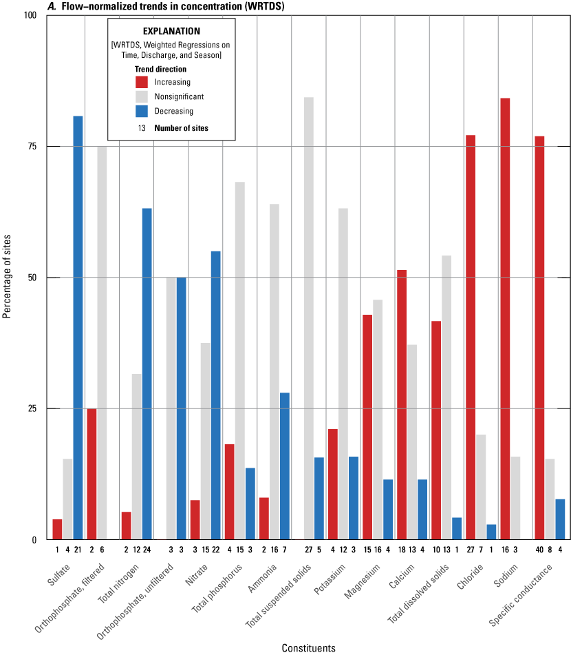
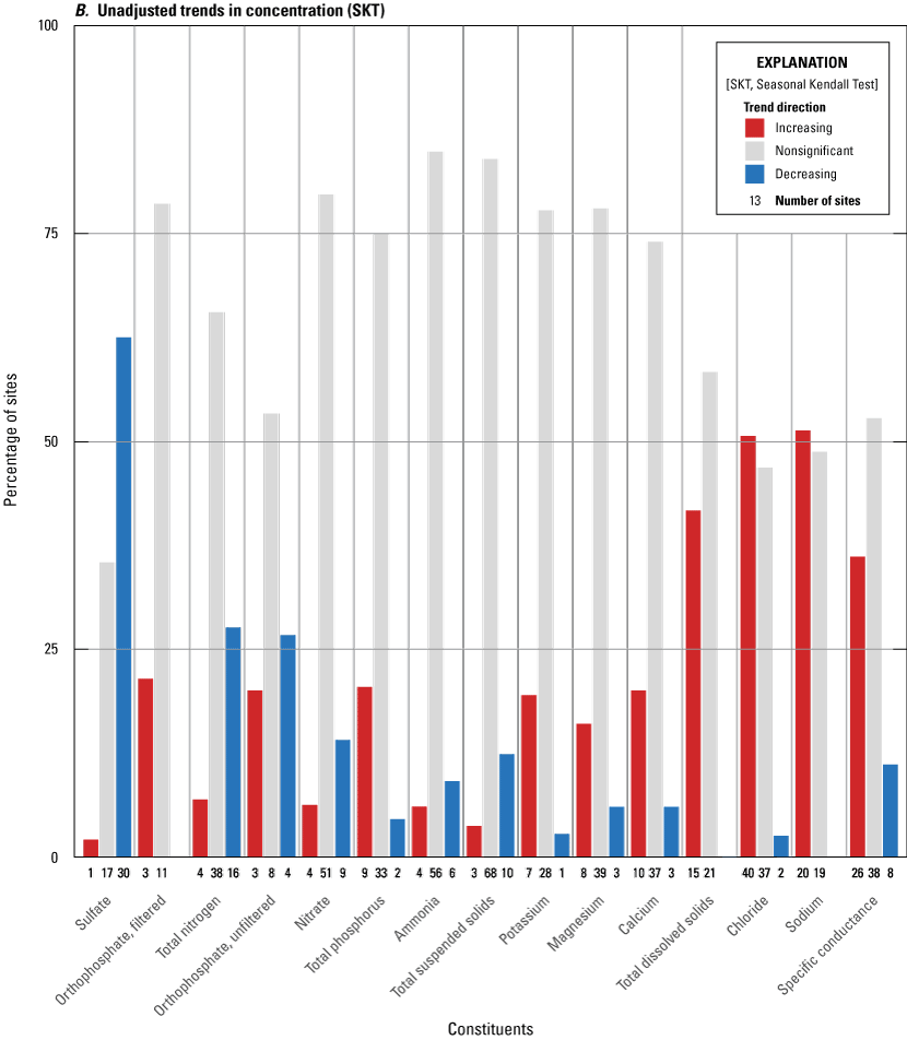
Percentage of sites with increasing, nonsignificant, and decreasing trends for each constituent for 2008–18 for A, flow-normalized trends in concentration calculated with Weighted Regressions on Time, Discharge, and Season and B, unadjusted trends in concentration calculated with the Seasonal Kendall Test.
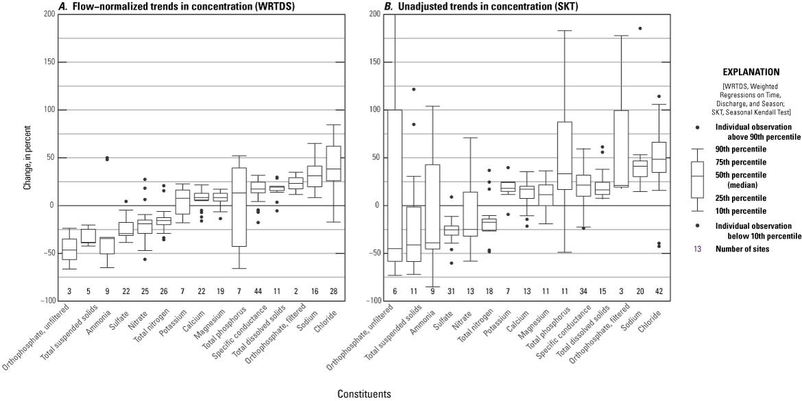
Percentage change of significant trends for each constituent, for A, flow-normalized trends in concentration calculated with Weighted Regressions on Time, Discharge, and Season and B, unadjusted trends in concentration calculated with the Seasonal Kendall Test for the 2008–18 trends. Percentage changes greater than 200 percent are not shown in these plots.
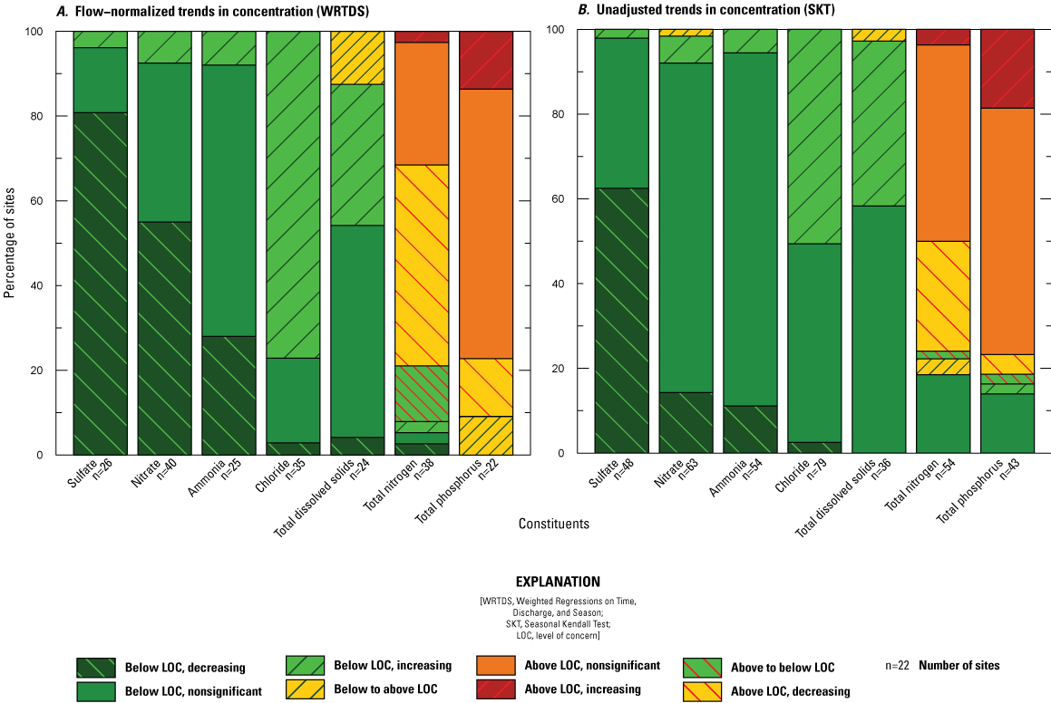
Percentage of sites for each constituent in the eight trend categories for A, flow-normalized trends in concentration calculated with Weighted Regressions on Time, Discharge, and Season and B, unadjusted trends in concentration calculated with the Seasonal Kendall Test, sorted based on the relation of the start and end concentrations of the 2008–18 trend to the level of concern and trend direction.
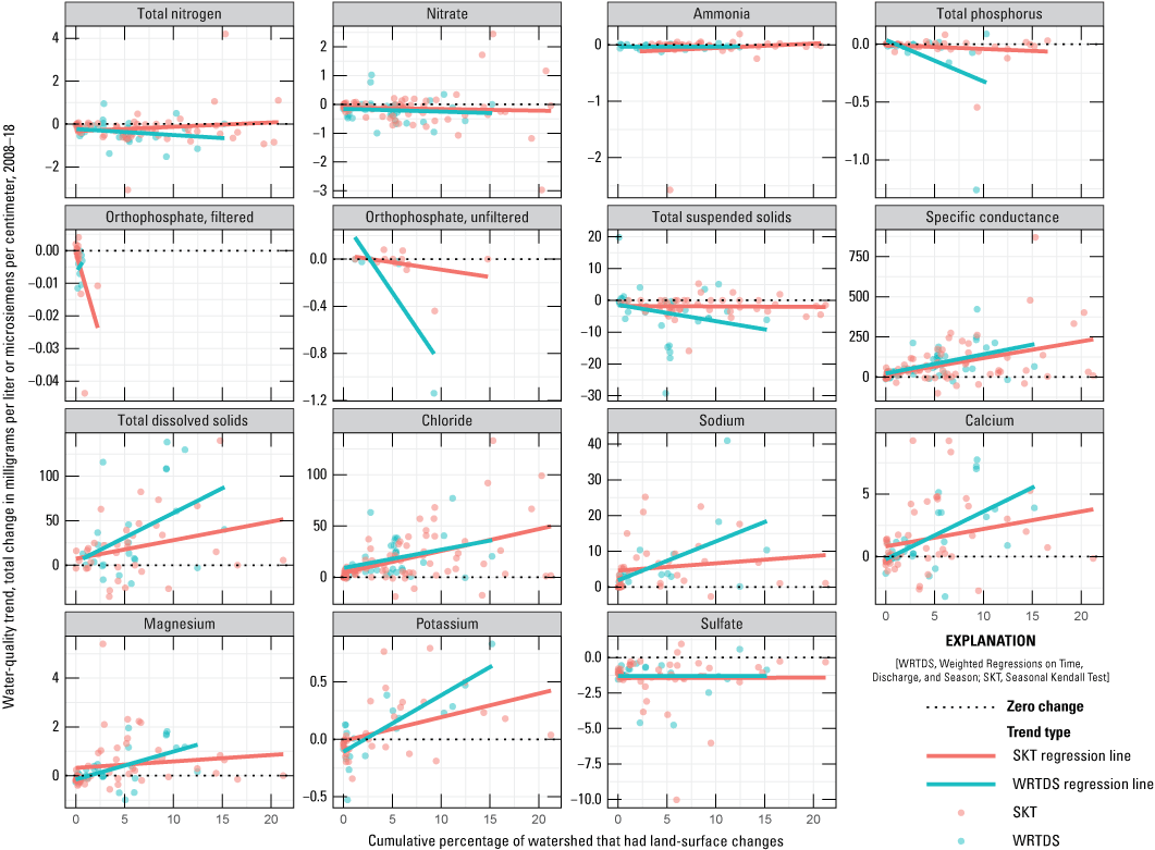
Total change of the 2008–18 water-quality trend versus the cumulative change in land-surface cover, as a percentage of the watershed, over the same period, by trend method type.
Spatial Distribution of Trends
The following maps (figs. 1.5–1.19) show the spatial distribution and the magnitude of the period of record trends for each constituent, with trends determined by the Seasonal Kendall Test and Weighted Regressions on Time, Discharge, and Season.
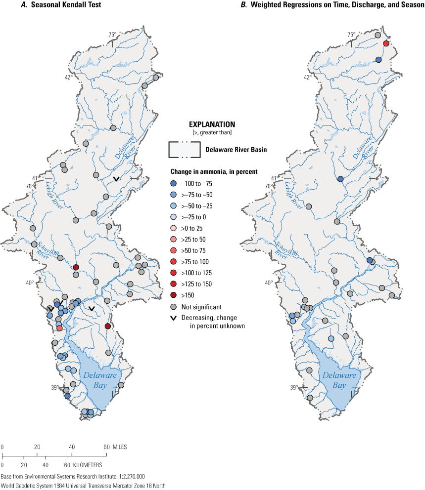
Sites with period of record trends for ammonia, determined by A, Seasonal Kendall Test (SKT) and B, Weighted Regressions on Time, Discharge, and Season (WRTDS).
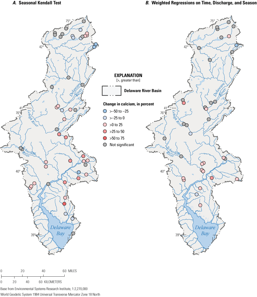
Sites with period of record trends for calcium, determined by A, Seasonal Kendall Test (SKT) and B, Weighted Regressions on Time, Discharge, and Season (WRTDS).
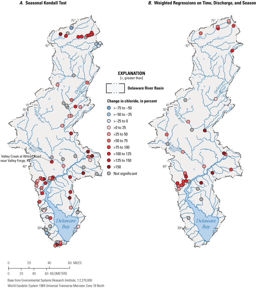
Sites with period of record trends for chloride, determined by A, Seasonal Kendall Test (SKT) and B, Weighted Regressions on Time, Discharge, and Season (WRTDS).
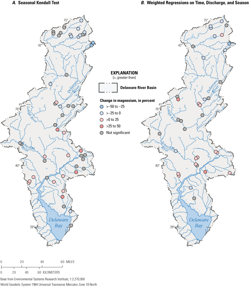
Sites with period of record trends for magnesium, determined by A, Seasonal Kendall Test (SKT) and B, Weighted Regressions on Time, Discharge, and Season (WRTDS).
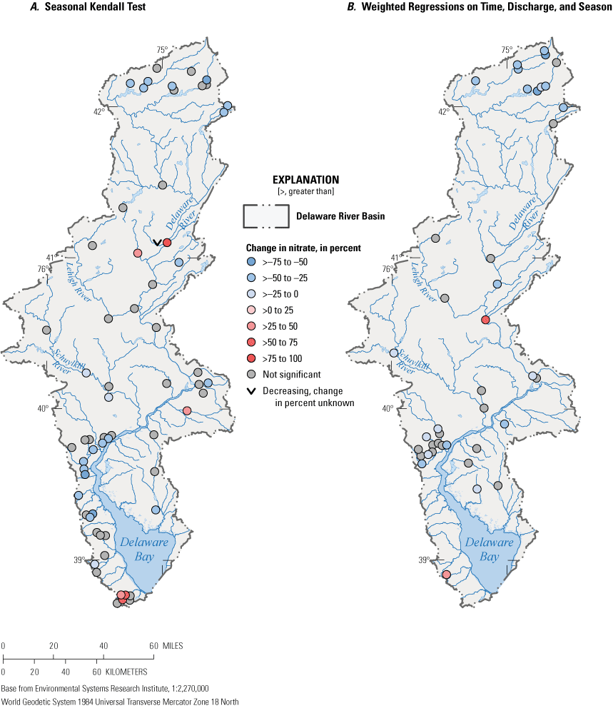
Sites with period of record trends for nitrate, determined by A, Seasonal Kendall Test (SKT) and B, Weighted Regressions on Time, Discharge, and Season (WRTDS).
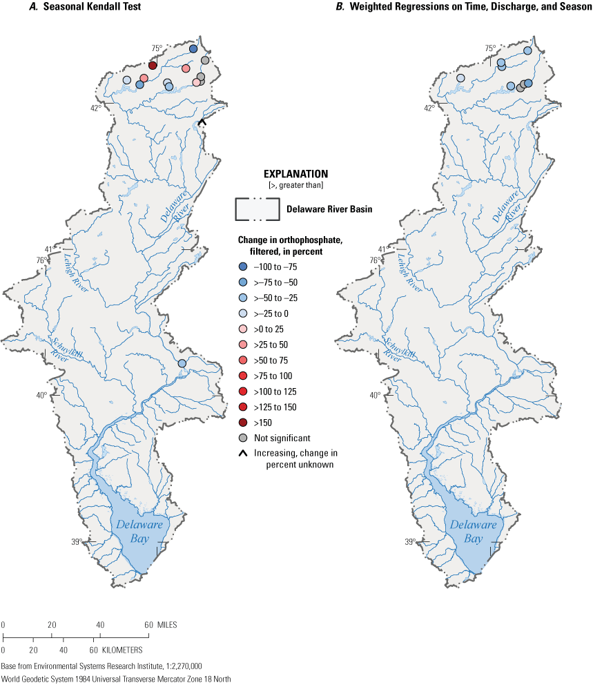
Sites with period of record trends for orthophosphate, filtered, determined by A, Seasonal Kendall Test (SKT) and B, Weighted Regressions on Time, Discharge, and Season (WRTDS).
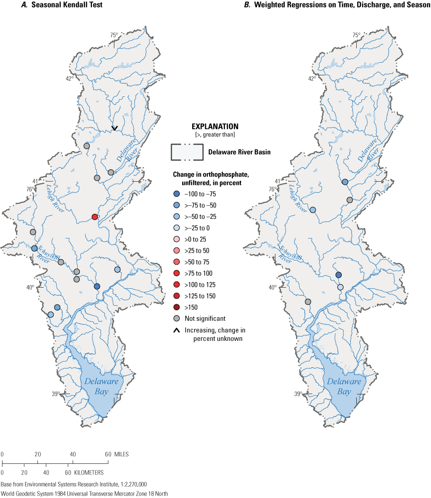
Sites with period of record trends for orthophosphate, unfiltered, determined by A, Seasonal Kendall Test (SKT) and B, Weighted Regressions on Time, Discharge, and Season (WRTDS).
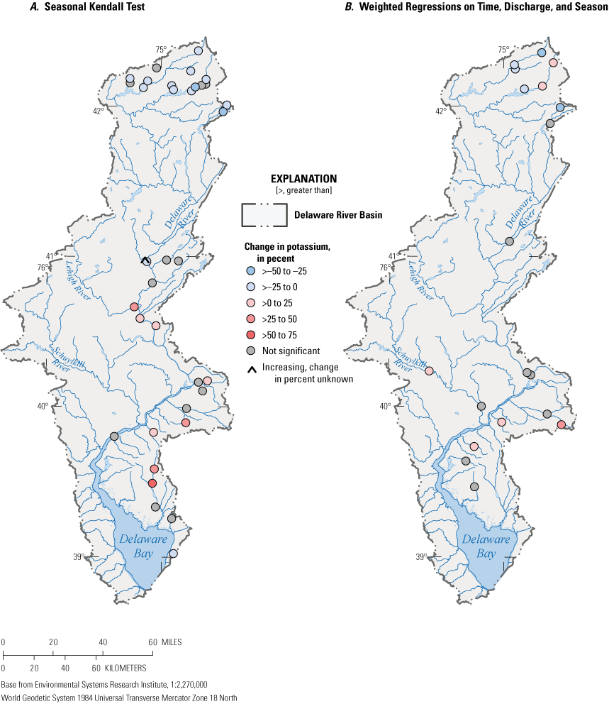
Sites with period of record trends for potassium, determined by A, Seasonal Kendall Test (SKT) and B, Weighted Regressions on Time, Discharge, and Season (WRTDS).
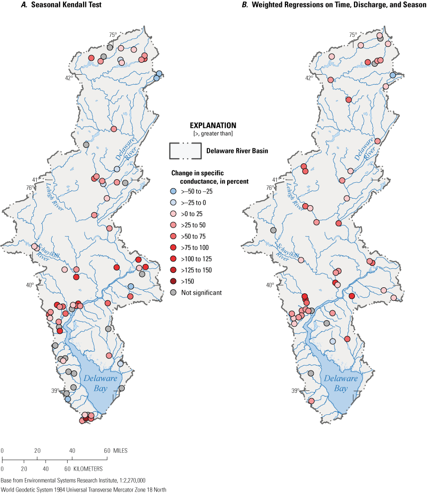
Sites with period of record trends for specific conductance, determined by A, Seasonal Kendall Test (SKT) and B, Weighted Regressions on Time, Discharge, and Season (WRTDS).
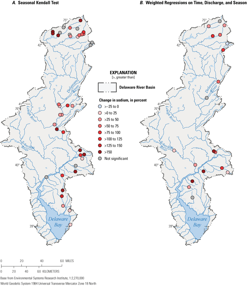
Sites with period of record trends for sodium, determined by A, Seasonal Kendall Test (SKT) and B, Weighted Regressions on Time, Discharge, and Season (WRTDS).
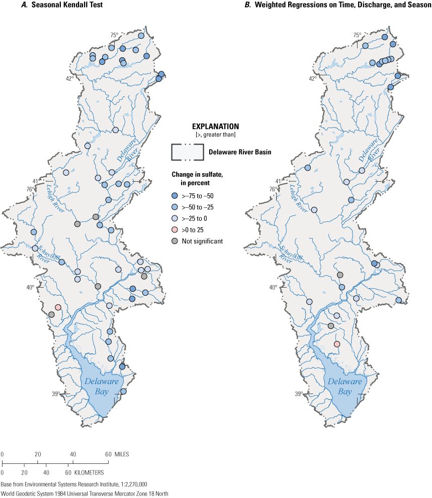
Sites with period of record trends for sulfate, determined by A, Seasonal Kendall Test (SKT) and B, Weighted Regressions on Time, Discharge, and Season (WRTDS).
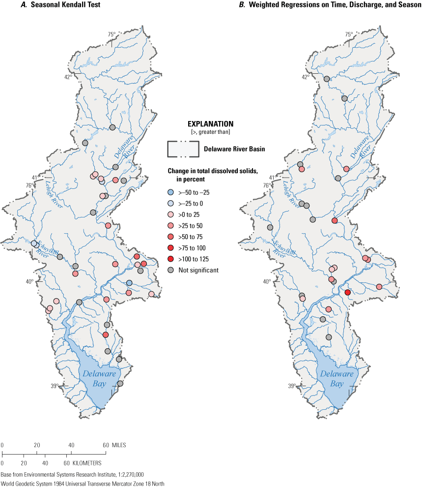
Sites with period of record trends for total dissolved solids, determined by A, Seasonal Kendall Test (SKT) and B, Weighted Regressions on Time, Discharge, and Season (WRTDS).
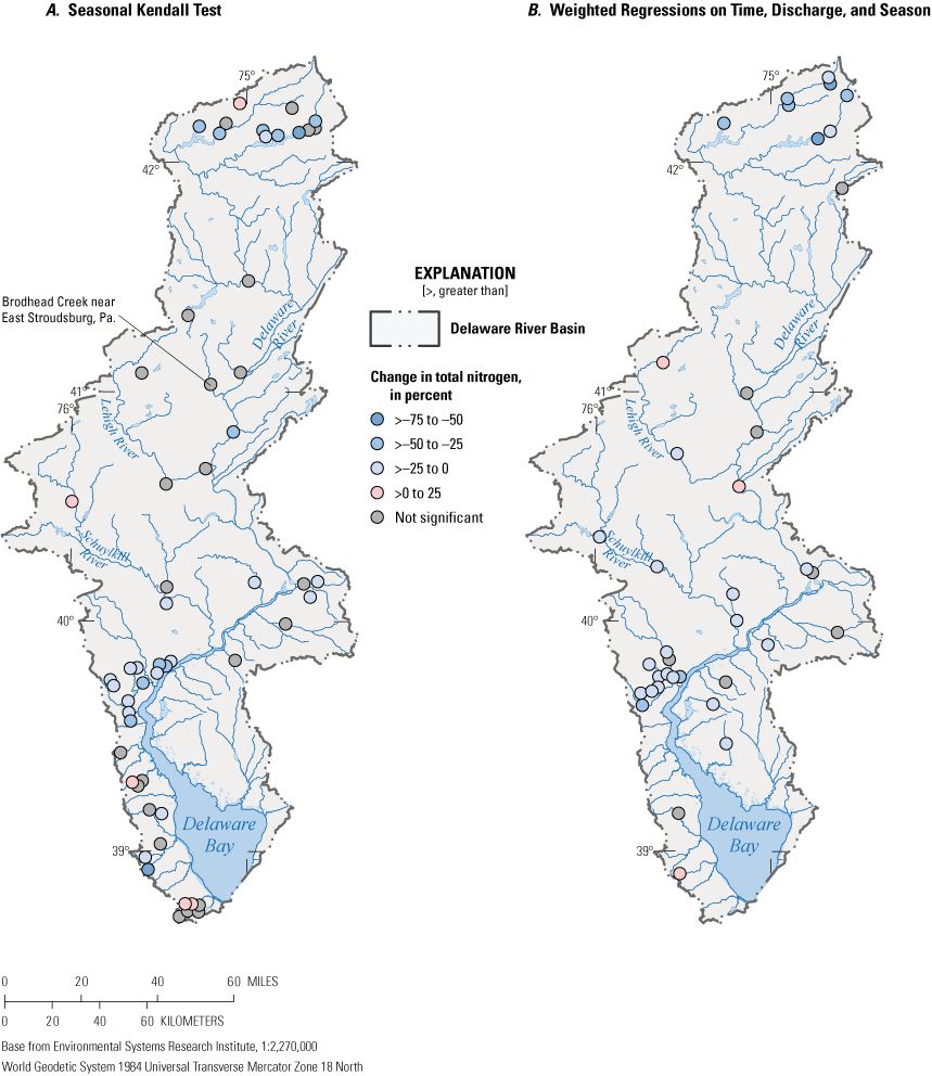
Sites with period of record trends for total nitrogen, determined by A, Seasonal Kendall Test (SKT) and B, Weighted Regressions on Time, Discharge, and Season (WRTDS).
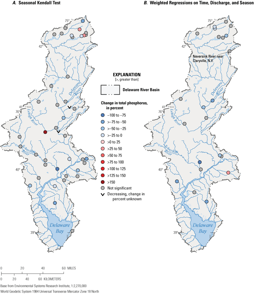
Sites with period of record trends for total phosphorus, determined by A, Seasonal Kendall Test (SKT) and B, Weighted Regressions on Time, Discharge, and Season (WRTDS).
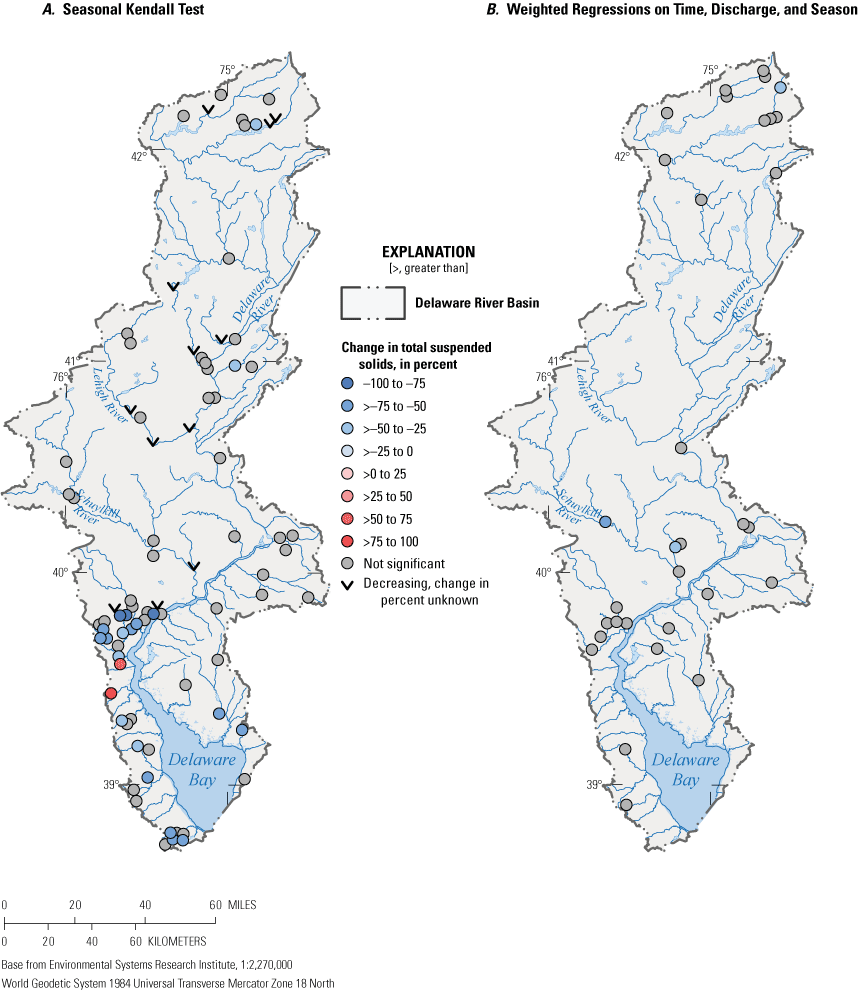
Sites with period of record trends for total suspended solids, determined by A, Seasonal Kendall Test (SKT) and B, Weighted Regressions on Time, Discharge, and Season (WRTDS).
Supplemental Comparison of Weighted Regressions on Time, Discharge, and Season and Seasonal Kendall Test Trends
For some sites, constituents, and trend periods, the criteria for both the Seasonal Kendall Test and Weighted Regressions on Time, Discharge, and Season were met, and trend results were generated with both methods. For the 993 results in which trend direction was available for both methods, 75 percent of the results agreed, generating significant trends in the same direction or nonsignificant trends with both methods. Table 1.2 presents the specific number of comparisons that fell into each trend direction group, by constituent. When the methods agreed, the absolute difference in percentage change by constituent varied (table 1.3).
Table 1.2.
Total number of trend results, for each constituent, determined by the Seasonal Kendall Test, and Weighted Regressions on Time, Discharge, and Season trend methods, and the number of results that fit into each comparison group.[SKT, Seasonal Kendall Test; WRTDS, Weighted Regressions on Time, Discharge, and Season]
Table 1.3.
Absolute difference in percentage change, for each constituent, between trend result pairs determined by the Seasonal Kendall Test and Weighted Regressions on Time, Discharge, and Season, when the trend direction was significant and in agreement.Supplemental Information
Specific conductance is given in microsiemens per centimeter at 25 degrees Celsius (µS/cm at 25 °C).
Concentrations of chemical constituents in water are given in either milligrams per liter (mg/L) or micrograms per liter (µg/L).
Abbreviations
FN
flow-normalized
IQR
interquartile range
LCMAP
Land Change Monitoring, Assessment, and Projection
LOC
level of concern
POR
period of record
SKT
Seasonal Kendall Test
SC
specific conductance
TDS
total dissolved solids
TN
total nitrogen
TP
total phosphorus
TSS
total suspended solids
USGS
U.S. Geological Survey
WRTDS
Weighted Regressions on Time, Discharge, and Season
For additional information contact:
Program Coordinator
U.S. Geological Survey
Water Availability and Use Science Program
National Water Quality Program
Email: wausp-info@usgs.gov
Publishing support provided by the Reston and West Trenton Publishing Service Centers
Disclaimers
Any use of trade, firm, or product names is for descriptive purposes only and does not imply endorsement by the U.S. Government.
Although this information product, for the most part, is in the public domain, it also may contain copyrighted materials as noted in the text. Permission to reproduce copyrighted items must be secured from the copyright owner.
Suggested Citation
Shoda, M.E., and Murphy, J.C., 2022, Water-quality trends in the Delaware River Basin calculated using multisource data and two methods for trend periods ending in 2018: U.S. Geological Survey Scientific Investigations Report 2022–5097, 60 p., https://doi.org/10.3133/sir20225097.
ISSN: 2328-0328 (online)
Study Area
| Publication type | Report |
|---|---|
| Publication Subtype | USGS Numbered Series |
| Title | Water-quality trends in the Delaware River Basin calculated using multisource data and two methods for trend periods ending in 2018 |
| Series title | Scientific Investigations Report |
| Series number | 2022-5097 |
| DOI | 10.3133/sir20225097 |
| Publication Date | December 12, 2022 |
| Year Published | 2022 |
| Language | English |
| Publisher | U.S. Geological Survey |
| Publisher location | Reston, VA |
| Contributing office(s) | Ohio-Kentucky-Indiana Water Science Center |
| Description | Report v, 60 p.; 2 Data Releases |
| Country | United States |
| State | Delaware, New Jersey, New York, Pennsylvania |
| Other Geospatial | Delaware River Basin |
| Online Only (Y/N) | Y |
| Additional Online Files (Y/N) | N |