

Field Techniques for the Determination of Algal Pigment Fluorescence in Environmental Waters—Principles and Guidelines for Instrument and Sensor Selection, Operation, Quality Assurance, and Data Reporting
Links
- Document: Report (4.03 MB pdf) , XML
- Related Works:
- Scientific Investigations Report 2022–5103 - Technical Note—Performance Evaluation of the PhytoFind, an In-Place Phytoplankton Classification Tool
- Techniques and Methods 1-D3 - Guidelines and standard procedures for continuous water-quality monitors: Station operation, record computation, and data reporting
- Download citation as: RIS | Dublin Core
Abstract
The use of algal fluorometers by the U.S. Geological Survey (USGS) has become increasingly common. The basic principles of algal fluorescence, instrument calibration, interferences, data quantification, data interpretation, and quality control are given in Hambrook Berkman and Canova (2007). Much of the guidance given for instrument maintenance, data storage, and quality assurance in Wagner and others (2006) are also applicable to algal fluorometers, although they are not explicitly discussed. Algal fluorometers have advanced substantially since these guidance documents were published; so that while the basic principles remain unchanged, new guidance is needed. This techniques and methods report is intended to provide additional information on algal fluorescence-sensor calibration, maintenance, measurement, data storage, and quality assurance that meet stated objectives of USGS data-collection efforts. The operations described facilitate and standardize the collection and accurate communication of algal fluorescence data collected by the USGS across studies, sites, and instrument types. This report provides technical background information on algal fluorescence sensors; including specifications, operating principles, key features, and design elements. Maintenance and calibration protocols, quality-assurance techniques, and suggestions for data reporting are presented. Sensor performance issues, common interferences, and strategies for addressing them are also described.
Introduction
Optical sensors that measure constituents in the environment by absorbance or fluorescence properties have a long history in limnologic and oceanographic research for measuring highly resolved concentrations and fluxes of algae, including cyanobacteria (also called blue-green algae), organic matter, and nutrients (Lorenzen, 1966; Vincent, 1983; Stauffer and others, 2019). For example, the development of in-place fluorometers for algal pigments over 50 years ago (Lorenzen, 1966) led to early advances in describing surface and depth patterns of phytoplankton in coastal oceans and lakes (Berman, 1972; Fee, 1976; Holligan and Harbour, 1977), and have become critical in understanding the spatiotemporal dynamics of harmful algal blooms in freshwater and marine environments (Lombard and others, 2019; Stauffer and others, 2019). Optical sensor technology is now sufficiently developed to warrant broader application for research and monitoring, and many water-quality programs are now collecting fluorescence data related to algal pigments (most often chlorophyll a and phycocyanin) using field-based sensors (Proctor and Roesler, 2010; Roesler and Barnard, 2013). However, collecting data that meet high-quality standards requires adherence to tested and established methods and procedures.
Fluorescence sensors require a greater understanding of sensor design, environmental interferences, algal dynamics, and limitations than many other sensors routinely deployed by the U.S. Geological Survey (USGS). Algal fluorescence sensors do not directly measure algal abundance, biomass, or pigment concentration, but rather the fluorescence response of algal pigments in the sample volume. For simplicity, sensors that measure the fluorescence response of algal pigments are called algal fluorometers throughout this document. The magnitude of fluorescence response can often, but not always, be related to algal pigment concentration (Falkowski and Kiefer, 1985; Gregor and Maršálek, 2004; Proctor and Roesler, 2010; Kasinak and others, 2015; Bertone and others, 2018, 2019). Fluorescence sensors can provide valuable insights into algal biomass and dynamics through relative patterns, and in some cases may be used as indicators of algal blooms (Kasinak and others, 2015; Lombard and others, 2019; Stauffer and others, 2019). However, because of sensor limitations and interferences, effective and consistent deployment requires thorough planning and setting realistic expectations for sensor performance and data objectives (Alliance for Coastal Technologies, 2017).
All algae contain the pigment chlorophyll a (chla), but there are many kinds of algae and each group has distinctly different accessory pigments (for example, chlorophylls b and c, carotenoids, and phycobilins, such as phycocyanin [PC] and phycoerythrin [PE]) that fluoresce at different wavelengths (Wetzel, 2001). Fluorescence can therefore be used as a proxy measurement for algal biomass or specific groups of algae. For example, a fluorometer can produce light at a particular wavelength (excitation) that causes the chla contained within algal cells to fluoresce at another wavelength (emission). The concentration of chla is generally proportional to the amount of chla fluorescence emitted (Lorenzen, 1966). Instruments targeting chla or PC (an indicator of cyanobacteria) are often used in fixed monitoring locations or in moving surveys in the aquatic environment (Alliance for Coastal Technologies, 2017; Bertone and others, 2018). Instruments with configurations that permit fluorescence measurements of several pigment types, and therefore several algal groups, are also available (Catherine and others, 2012; Alliance for Coastal Technologies, 2019a–d; Johnston and others, 2022).
It is important to have a realistic expectation of the kinds of information algal fluorometers can provide. There may be general proportional relations between pigments and the abundance of algae or algal groups; however, measured fluorescence per unit of chla or other algal pigments can vary up to severalfold based on influences including physiological status, cell morphology, temperature, light, and photoinhibition (Catherine and others, 2012; Alliance for Coastal Technologies, 2017, 2019a–d Bertone and others, 2018, 2019; Proctor and Roesler, 2010; Roesler and Barnard, 2013; Johnston and others, 2022). As such, field-based measurement of algal fluorescence should not be considered a quantitative measure, but rather a relative measure that can be used to evaluate potential spatial or temporal changes in algal abundance or community composition or both. Proportional relations may be difficult to determine at some locations, but relative patterns can provide useful insights, depending on the study objectives. In some cases, fluorescence measurements may be used more quantitatively if the relation is supported with extractive laboratory analysis or algal identification and enumeration (also known as population counts).
This techniques and methods report is intended to provide additional information on algal fluorescence sensor calibration and maintenance, measurement, data storage, and quality assurance that meet stated objectives of USGS data-collection efforts. The basic principles of algal fluorescence and instrument calibration, interferences, data quantification, data interpretation, and quality control are given in the National Field Manual for the Collection of Water-Quality Data, book 9, chapter A7.4 “Algal Biomass Indicators” (Hambrook Berkman and Canova, 2007). Much of the guidance given for instrument maintenance, data storage, and quality assurance in USGS Techniques and Methods book 1, chapter D3 (“Guidelines and Standard Procedures for Continuous Water-Quality Monitors—Station Operation, Record Computation, and Data Reporting,” Wagner and others, 2006) is also applicable to algal fluorometers, although they are not explicitly discussed. Algal fluorometers have advanced substantially since these guidance documents were published; so that while the basic principles remain unchanged, new guidance is needed.
Purpose and Scope
The purpose of this report is to provide information on the selection and use of field fluorescence sensors (also referred to as “field fluorometers”) by the USGS for in-place determination of the presence, relative abundance, and qualitative estimates of algal pigment concentrations in environmental waters. This report will help USGS personnel and others collect field data by using algal fluorometers in ways that are consistent and comparable across studies, sites, and instruments. For those who have selected fluorometric instrumentation for measurement of algal pigments in the field, this report provides guidance on instrument preparation and deployment, ongoing maintenance and field operations, quality-assurance procedures, and data reporting. This report supplements manufacturer user manuals for individual sensors. This report will not aid in quantifying or correcting for the various interferences discussed within. Quantifying and correcting for these interferences warrant their own investigations and these topics are beyond the scope of this report.
Related Information
The following section was modified from Pellerin and others (2013).
This report is designed to supplement other USGS documents describing collection and reporting of water-quality data, including the deployment and use of continuous water-quality monitors. The following is a list of related USGS publications that are presented in order of general to more specific guidelines:
U.S. Geological Survey Fundamental Science Practices.—The Fundamental Science Practices (FSPs; U.S. Geological Survey, 2018a) are a collection of policies in the USGS Survey Manual that ensure the quality and integrity of USGS science, including procedures for planning and conducting data collection and research (chapter 502.2; U.S. Geological Survey, 2011), peer review (chapter 502.3; U.S. Geological Survey, 2016a), and review, approval, and release of information products (chapter 502.4; U.S. Geological Survey, 2016b). This report facilitates adherence to FSPs by providing specific guidelines for the deployment, maintenance and field operations of algal fluorometers, and data quality assurance and reporting.
U.S. Geological Survey Quality Management System Instructional Memorandum 2018–01 and Quality Management System Manual (version 2.0).—This USGS Quality Management System (QMS) memo (U.S. Geological Survey, 2018b) and manual (U.S. Geological Survey, written commun., 2021) provides a foundation to ensure that laboratory activities, including instrument checks and calibrations, meet a defined standard of quality. The report facilitates adherence to the QMS by providing specific guidelines for the documentation of laboratory check and calibration of algal fluorometers.
U.S. Geological Survey National Field Manual for the Collection of Water-Quality Data.—The National Field Manual (U.S. Geological Survey, variously dated) provides information and guidelines on preparing for sampling, selecting, and cleaning equipment, collecting, and processing water samples, and taking field measurements. Much of the information is directly applicable to deploying algal fluorescence sensors and collecting the metadata needed for interpreting the results. Chapters A1 to A6 (Wilde, variously dated b, variously dated c, 2004; Wilde and others, 2014; U.S. Geological Survey, 2006, 2018d) provide critical information on preparing for water sampling, selection and cleaning of sampling equipment, sample collection, and methods for making ancillary field measurements that are useful for understanding algal fluorescence sensor results, such as temperature, dissolved oxygen, specific conductance, pH, and turbidity. Chapter A7 (Wilde, variously dated a) includes guidelines for the determination of biological indicators including algal biomass (chap. 7.4, Hambrook Berkman and Canova, 2007) and cyanobacteria (chap. 7.5, Graham and others, 2008) in surface waters. Chapter A10 (U.S. Geological Survey, 2018c) presents guidance for sampling lakes and reservoirs and includes discussion of basic limnological principles, algal biomass, and cyanobacteria. Personnel who use algal fluorescence sensors can benefit from a solid understanding of the guidelines provided in these chapters.
Techniques and Methods book 1, chapter D3, Guidelines and Standard Procedures for Continuous Water-Quality Monitors: Station Operation, Record Computation, and Data Reporting.—This report (Wagner and others, 2006) provides basic guidelines and procedures for use by USGS personnel for site and water quality instrument selection, field procedures, calibration of continuous water-quality monitors, record computation and review, and data reporting. Although the use of algal fluorescence sensors requires specific guidelines beyond those provided in the chapter, the general workflow for their use is similar to the workflow described within for basic sensors. The terminology and processes described thus form the general background for the use of algal fluorescence sensors.
Techniques and Methods book1, chapter D5, Optical Techniques for the Determination of Nitrate in Environmental Waters: Guidelines for Instrument Selection, Operation, Deployment, Maintenance, Quality Assurance, and Data Reporting.—This chapter (Pellerin and others, 2013) provides information about the selection and use of ultraviolet (UV) nitrate sensors by the U.S. Geological Survey to facilitate the collection of high-quality data across different studies, sites, and instrument types. Although the focus of the chapter is UV nitrate sensors, many of the principles can be applied to other in-place optical sensors for water-quality studies.
U.S. Geological Survey Water Resources Division Policy Memorandum 2010.02 and Office of Water Quality Technical Memorandum 2017.02.—The Water Resources Division (renamed as the Water Mission Area [WMA]) memorandum (U.S. Geological Survey, 2010) specifies a schedule for the review and approval of time-series data collected in support of USGS activities. The Office of Water Quality (OWQ) memorandum (U.S. Geological Survey, 2017) clarifies the appropriate justification for time-series records and site category assignment (categories 1, 2, and 3). USGS personnel should seek out policy updates or changes before beginning new data collection efforts to ensure that references used are up to date, and all current (2022) policies are being followed.
Principals of Light and Algal Pigment Fluorescence
The transmission of light through water is altered by the physical and chemical properties of the constituents within it (fig. 1). Light scattering and light absorption are two processes that affect algal pigment measurements. Light scattering is a process where radiant or light energy (also referred to as photons) is redirected in multiple directions primarily by particles and forms the basis for measurements such as turbidity, which will only be discussed in this report in the context of signal interference (see section “Interferences Affecting In-Place Measurements of Algal Pigment Fluorescence”). Light is absorbed when light energy is converted into nonradiant energy by exciting an electron from a ground state atomic orbital to a higher energy atomic orbital. Absorbed energy is then released through multiple competing pathways that include nonradiative thermal pathways such as vibrational relaxation and nonradiative decay, and in the form of fluorescence (near-instantaneous emission) and phosphorescence (delayed emission) as the excited electron returns to the ground state atomic orbital. Fluoresced light is always emitted with less energy and therefore at longer wavelengths than the absorbed light—a phenomenon known as the Stokes shift (fig. 2; Stokes, 1852).

Conceptual diagram of light scattering and absorption by particles or dissolved constituents in water. The inset Jablonski diagram shows how a fluorophore such as chlorophyll a absorbs shorter wavelength ultraviolet light (blue arrow) and releases energy as fluorescence at longer wavelengths (red arrow) and nonradiative decay (gray arrow).

Conceptual graph showing light excitation and emission wave properties of a theoretical substance.
The phenomenon of fluorescence can be observed with a wide variety of substances in water, ranging from living algae and organic compounds leached from plants and animals to synthetic compounds from oil, grease, dyes, and optical brighteners used in laundry detergents. Properties of the chemical bonds within the fluorescing material (known as fluorophores) determine the wavelengths at which light is most strongly absorbed and at which wavelengths light is emitted as fluorescence. Because these wavelengths are specific, it is often possible to make measurements of targeted substances within the complex mixture of absorbing and fluorescing materials found in environmental waters by providing a light source at the wavelengths that correspond to absorption and emission maxima characteristic to that substance. For more detail on the chemistry and physics of fluorescence and absorbance, see the numerous reviews by Guilbault (1990), Maxwell and Johnson (2000), Lakowicz (2006), Suggett and others (2010), Coble and others (2014), and Bertone and others (2018).
Measuring Algal Pigment Fluorescence
All algae contain chlorophyll a (chla), a water-insoluble, light-harvesting pigment involved in photosynthesis that emits approximately 3–5 percent of the absorbed light energy in the blue and red regions of the light spectrum as fluorescence (Falkowski and Kiefer, 1985). Chla is not simply contained within the cell, but rather, it is associated with biomolecules and packaged within cellular thylakoid membranes in ways that lead to variability in the peak absorption and emission bands as well as the relative fluorescence emissions (Roesler and Barnard, 2013). These variations in the chemical properties of chla also affect the intensity of measured fluorescence per unit of chla (commonly referred to in literature as “fluorescence yield”), which can vary several-fold based on the algal species and physiological status of cells (Proctor and Roesler, 2010; Roesler and Barnard, 2013).
Measurement of algal fluorescence using field-based sensors may be referred to as “in place” (within the original position of the sample, commonly called “in situ”) or “in body” (within the body or cells of a living organism, commonly called “in vivo”). “In-body fluorescence” is often used to refer to fluorescence measured from intact, living algae, which range in linear size from <0.2 micrometer (µm; picoplankton) to >2 millimeters (mm; macroplankton). To distinguish between laboratory-based approaches that may be used to measure fluorescence of live algae, field-based sensor measurements are referred to as “in place measurements” throughout this report. In contrast to in-body measurements, extracted (also called “in vitro”) measurements are laboratory-based fluorescence measurements typically made on samples of algae that are no longer living and have been collected on a filter and the pigments extracted with an organic solvent. Because extracted measurements are made on pigments dissociated from various proteins and membranes within living cells, the resulting fluorescence is typically higher than the observed in-body fluorescence (Hambrook Berkman and Canova, 2007). The relations between algal pigment-fluorescence measured in extracted samples of algae and by in-place sensors vary across hydrologic systems, algal species, sample depth, and even time of day; therefore, if the purpose of monitoring is to quantify pigment concentrations, each system should be evaluated independently.
In addition to chla, there are other fluorescent accessory pigments including chlorophylls b, c, and d, carotenoids, xanthophylls, and phycobilins (for example, phycocyanin and phycoerythrin) which are used by algae to harvest and shuttle photons from sunlight to make energy. Whereas all algae; including cyanobacteria, green algae, and diatoms contain chla; accessory pigments can be diagnostic of the different types of algae present (Wetzel, 2001). This is possible to measure because these pigments vary in their light absorption spectra, or how they absorb (and therefore use) or reflect light, at different wavelengths (fig. 3).

Graph showing absorption spectra of plant pigments. Figure by Boundless, licensed under Creative Commons Attribution-ShareAlike 4.0 International Public License, https://creativecommons.org/licenses/by-sa/4.0/legalcode, found at https://bio.libretexts.org/Bookshelves/Introductory_and_General_Biology/Book%3A_General_Biology_(Boundless)/08%3A_Photosynthesis/8.05%3A_The_Light-Dep endent_Reactions_of_Photosynthesis_-_Absorption_of_Light.
Together, the absorbed light and ensuing fluorescence produce characteristic excitation–emission maxima, or wavelength peaks, per different pigments. These wavelengths can be detected, quantified, and used to estimate pigment concentration using multiwavelength scans, or with single or dual wavelength sensors in a targeted manner. Chlorophyll a has a primary absorption peak in the blue (at about 430 nanometers [nm]) part of the visible light spectrum, and a smaller, secondary peak in the red part (at about 660 to 665 nm); plants are green because they reflect light in the green part of the spectrum (Wetzel, 2001). Cyanobacteria are of particular interest because of their potential to form harmful algal blooms (Graham and others, 2008). Important secondary pigments in cyanobacteria are the phycobilins PC and PE, which have peak absorption at fluorescence wavelengths near 595 nm and 670 nm, and 528 nm and 573 nm, respectively (Hambrook Berkman and Canova, 2007).
Fluorescence as a Proxy for Algal Biomass and Community Composition
Chla is a near-universal proxy for algal biomass (Wetzel, 2001; Hambrook Berkman and Canova, 2007). Fluorescence sensors do not directly measure chla or other algal pigments, but rather measure a relative fluorescence response of a whole water sample at a specific absorption wavelength. Measurement of pigments other than chla can give an indication of the presence and abundance of other algal groups of interest, such as cyanobacteria, or broader algal community composition. Fluorescence response is often (but not always) proportional to pigment concentration in water, and can be used, for example, to estimate chla or PC concentration. The fluorescence measurements described in this report are commonly compared to laboratory-measured concentrations of chla (most commonly, chla in micrograms per liter [µg/L]), to PC or PE (also in µg/L), or to the abundance or biovolume of total algae or specific algal groups (in cells per liter or biovolume per liter). This proxy-based relation between the in-place sensor measurement and the laboratory-measured quantity of interest is in contrast to sensors that make more direct measurements such as optical nitrate sensors; the magnitude of the absorbance at a peak wavelength (for example, 220 nm for nitrate) is directly proportional to the concentration of ions in solution (Pellerin and others, 2013). Users of algal fluorometers must be aware that algal fluorescence is a proxy (or indirect) measure and may not always be directly proportional to concentrations of chla or other pigments of interest.
Many factors influence the fluorescence response of living algae and can cause variability in the relation between in-place sensor measurements and extraction-based measurements in the laboratory (fig. 4). For example, not all taxa have the same amount of pigment and some taxa are more efficient at harvesting and using light, resulting in order-of-magnitude variability in chla fluorescence yields (Vincent, 1983; Proctor and Roesler, 2010; Roesler and Barnard, 2013; Bertone and others, 2018) that represent one of the largest sources of variability in the relation between field and laboratory-measured pigment concentrations (Roesler and Barnard, 2013; Proctor and Roesler, 2010). Another factor that causes variability in fluorescence yield is the general health of algae (Olaizola and others 1994), which affects the overall amount and type of pigments produced and hence their fluorescence. In addition, fluorescence may exhibit extreme diurnal variability caused by nonphotochemical quenching, resulting in apparent changes in pigment concentrations that are not indicative of changes in biomass concentration (Beutler and others, 2002; Roesler and Barnard, 2013; Bertone and others, 2018).
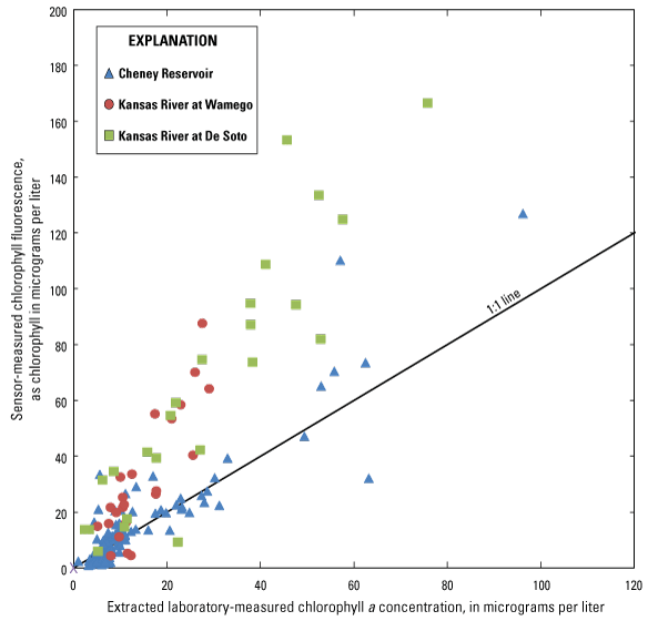
Sensor-measured chlorophyll fluorescence, as chlorophyll concentration, compared with laboratory-measured extracted chlorophyll a concentration (uncorrected) in discretely collected samples at three sites in Kansas (Cheney Reservoir near Cheney Kansas, U.S. Geological Survey Station 07144790, October 2008–October 2014; Kansas River at Wamego, Kansas, U.S. Geological Survey Station 06887500, July 2012–December 2014; Kansas River at De Soto, U.S. Geological Survey Station 06892350, July 2012–December 2014). Fluorescence sensors were calibrated using rhodamine WT dye. Data are from U.S. Geological Survey (2016c).
Although sensor-based measures of algal fluorescence may not always be directly related to concentrations of algal biomass or algal pigments, patterns in algal fluorescence contain inherently valuable information that can indicate the following:
-
• health of an algal population (strong diurnal fluctuations in fluorescence may be indicative of a healthy algal population, Olaizola and others, 1994);
-
• spatial variations in concentration (relative fluorescence may indicate horizontal and vertical changes within and among systems);
-
• temporal changes in concentration (increasing relative fluorescence over a period of days or weeks may be indicative of increased concentrations);
-
• dominant algal group (for example, an increase in the ratio of PC fluorescence to chlorophyll fluorescence may indicate increased dominance by cyanobacteria); and
-
• whether streamflow- or biology-based processes are dominant in lotic (rapid freshwater) ecosystems (for example, diurnal patterns in algal fluorescence may be dampened when streamflow-based process are dominant relative to periods when biology-based processes are dominant).
Sensor Design
The overall design of commercial field fluorometers is generally similar among manufacturers and includes features for physical configuration, optics, and data processing. However, the configuration may affect the instrument range, resolution, and the tolerance for interferences. A clear understanding of differences in the configuration and data output specifications will help with choosing the appropriate fluorometer for different aquatic environments and applications. Typically, the manufacturer’s instrument documentation will contain relevant information on design and specifications to choose a field fluorometer that best meets study needs.
Basic Sensor Design
In-place fluorometers generally work as follows: a light-emitting diode (LED) is used to generate a nearly monochromatic beam of light at a predetermined wavelength, and the light passes through a water sample of known dimensions and volume that is internal or external to the sensor body (fig. 5). A photodetector measures light returned from responsive fluorophores present in the sample at nearly the same time that it was emitted, as the process of fluorescence is nearly instantaneous (with a delay of only one hundred billionth to one hundred millionth of a second; Guilbault, 1990; Suggett and others, 2010). The specific wavelengths of fluoresced light measured by the sensor’s photodetector are determined by optical filters embedded within the sensor housing. After additional, instrument-specific filtering or processing of the light-derived electronic signal or both, a measurement is calculated in volts or counts and transmitted in analog or digital format (for example, Recommended Standard 232 [RS-232], serial-digital interface at 1200 baud [SDI-12], or Recommended Standard 485 [RS-485]) to a data-collection platform (DCP) for logging or transmission. The collected data can then be converted to other fluorescence or concentration units based on manufacturer or calibration-defined scale factors.

Schematic showing the general configuration of open-face (left) and flow-through (right) fluorometer designs.
The physical components of field and laboratory fluorometers are essentially the same, and include a light source, optical filters, and a photodetector. Critical to the function of each component are the associated electronic circuits that include regulated power supplies, lamp drivers, instrumentation amplifiers, analog-to-digital converters, and a microcontroller programmed for the desired output format and data preprocessing. Some sensors are equipped with adjustable (as opposed to automatic) gain settings that can be used to maximize the linear range, which may be useful for specific applications at the low or high end of the dynamic range. However, a number of important physical modifications are necessary when laboratory fluorometers are miniaturized and adapted for field deployments. Modifications include the use of low-power LEDs as a light source instead of high-intensity xenon or mercury lamps, and elimination of the excitation monochrometer typically used in benchtop fluorometers for scanning across a range of excitation and emission wavelengths. These and other modifications, including ruggedized, waterproof housings and solid-state electronic components (such as integrated circuit boards and transistors which have no moving parts), efficient power and heat handling, and antifouling components, not only affect the ability to make accurate fluorescence measurements in place, but also affect the serviceability, longevity, stability, and cost of field fluorometers.
The light source in the current (2022) generation of field fluorometers is typically composed of one or more LEDs, which reduces the cost, power consumption, longevity, and size of instruments relative to other types of lamps used in field spectrophotometers (such as deuterium and xenon flash lamps). When excited by light emitted by LEDs, the stability, lifetime, and quantum yield (ratio of photons emitted to photons absorbed) of fluorophores varies by wavelength; but measurements of chla and PC excitation by LEDs indicate little drift even over thousands of hours of operation. Photodetectors are the true sensing elements of the instrument and, typically, are photodiodes or diode arrays characterized by low cost, low power consumption, and small size. The angle at which the excitation light source and the emission detector are placed relative to each other (typically from 90 to 140 degrees) determines the sample volume; the volume is geometrically defined by where the excitation light beam intersects with the cone of reception of the detector (fig. 5). As the acceptance angle or detection cone is increased, the length of the sample volume and the amount of light attenuated along the sample path is decreased. Attenuation of received light can be caused by particles scattering the light along the sample path, and by photons reabsorbing the fluoresced light within the sampling volume. Optical filters are made of glass or other materials that filter out unwanted wavelengths emitted from the light source, and from fluoresced light returning to the detector. Bandpass filters used in most field fluorometers typically allow for a broad spectral distribution. The common specifications of bandpass filters are the wavelength with peak transmittance, the peak center wavelength (the average of two half-height wavelengths in a spectrum) and the peak wavelength full width at half maximum (the wavelength at half of the maximum transmittance; fig. 2).
All field fluorometers are equipped with an electronic signal processor that converts the raw current from a photodetector to a useful measurement output. Instruments can use a system of analog and digital electronic circuits, or a specialized microcontroller known as a digital signal processor to detect, convert, and emit signals at very high internal sample frequencies, which are then integrated to output high-frequency data (from 1 to 20 hertz [Hz]) by an analog or digital (RS-232) signal output. A microcontroller also controls the modulation of the LED so that the system can detect and differentiate between fluorophores and background noise (that is, photodetector dark current). Some sensors may employ dynamic gain to increase sensitivity and prevent saturation over a broader range of conditions. Most field fluorometers are designed to be integrated with external DCPs that provide power to the sensors and a datalogger controller to record the output of the fluorometer. Field fluorometers equipped with digital output in the form of serial communication (for example, RS-232, RS-485, USB or SDI-12) are common and desirable compared to analog output fluorometers for most continuous-monitoring deployments. Although there are many other protocols for serial communication, the majority of DCPs currently in use are designed to directly interface using RS-232, SDI-12 and RS-485 serial protocols.
Sensor Specifications
Field fluorometers are typically characterized by the three following data-quality specifications: (1) detection limit, (2) dynamic range (typically within the linear range of the sensor), and (3) resolution. Currently (2022), there are no accepted national or international standards to which these measurements can be compared, such as those available for other water quality measurements published by the National Institute of Standards and Technology (NIST) or the International Organization for Standardization (ISO). In addition, the accuracy of field fluorometers is the degree of agreement between the sensor-measured and true-fluorescence intensity, which is primarily affected by two sources of uncertainty: (1) instrument noise and (2) interferences. Although instrument noise; which is caused by the electronic components, the light source, and the detector resolution; is often random (Skoog and others, 2007), a systematic error can result in good precision but poor accuracy (that is, bias). Therefore, instruments with low electronic noise and a greater tolerance (that is, lower uncertainty because of matrix interferences) for interferences from suspended particles or dissolved organic matter (DOM) have greater accuracy. However, it is important to recognize that these specifications relate to the fluorescence measurements themselves; they do not reflect the correlation of the measurement to laboratory-measured pigment concentrations, algal abundance, or algal community composition.
In addition, manufacturer specifications are often determined under controlled operating conditions, averaged for a limited number of sensors, and by using primary reference materials (for example, an algal culture of a single species) in solutions that typically result in greater accuracy, greater precision, and lower detection limits than would be observed if measured in environmental waters where interferences are a factor. The results are then sometimes scaled across a range using an algorithm and secondary reference materials (for example, rhodamine WT, see Smith, 2020). Individual sensors can vary in performance because of even small variations in the manufacturing process. Prior to deploying an instrument in the field, it is important to independently verify instrument performance in a controlled environment, such as a laboratory, with appropriate standards and interferences (such as suspended particles and DOM). The baseline performance data collected prior to deployment serves as a basis for evaluating instrument performance after deployments and during instrument servicing.
The detection limit for fluorometers can be defined as the lowest value measurable by a given sensor that can be distinguished from a blank value with some level of statistical confidence (usually 99 percent; 40 CFR §136 app. B). Detection limits for in-place fluorometers are a function of both the detector sensitivity and the instrument electronic noise. In general, the detection limits of the current (2022) generation of in-place fluorometers are very low in environmental waters and may be important for waters with low levels of algal pigments.
The dynamic range is defined as the difference between the lowest and highest concentrations that can be measured, although the range over which the instrument response is linear (linear dynamic range) is often of greater interest. Linearity is typically reported by the manufacturer as the coefficient of determination, r2, or can be determined by users from a calibration curve across the dynamic range. The maximum detectable value is particularly important for fluorometers, especially when used in systems with excessive algal biomass or algal blooms, and is determined by several factors including the chemical composition of the target constituent and the instrument’s optical path length and components. Some sensors are equipped with adjustable (as opposed to automatic) gain settings that can be used to maximize the linear range, which may be useful for specific applications at the low or high end of the dynamic range.
Instrument resolution is defined as the minimum difference between measured values reliably detected by the sensor. The current (2022) generation of field fluorometers can typically measure at a resolution of two decimal places.
Factors Influencing Observed Fluorescence
Fluorescence is an inherent property of many substances that can exist in environmental waters. As such, there are several processes that influence fluorescence response, and may cause substantial variability. Additionally, as with all optical sensors, it is critical to account for light-absorbing or light-scattering materials present in the sample that interfere with light transmission to a detector. Collectively, these are known as “matrix effects” because they result from properties of the matrix, the surrounding material in which the measurement of fluorescence is being made (Pellerin and others, 2013). It is important to have a thorough understanding of these processes and matrix interferences to distinguish them from other factors that may interfere with in-place measurements of algal fluorescence.
Processes Affecting Fluorescence Response
Several environmental and chemical variables affect fluorescence response because they affect the capacity of the fluorescing molecule to dissipate energy, which thereby reduces detectable excitation. These effects are referred to as photochemical quenching. Nonphotochemical quenching, a form of dissipation of absorbed light employed by plants and algae to protect themselves from high light intensity, is a commonly observed effect specific to fluorometric measurement of algal pigments.
Photochemical Quenching
The most common form of photochemical quenching is related to temperature. Temperature is inversely related to fluorescence; the collisions of molecules at higher temperatures experience energy loss through kinetic interactions, which affords an easier path for energy loss than fluorescence. Simply put, as temperature increases, fluorescence decreases (Guilbault, 1990). Temperature corrections for algal fluorescence can be applied but may be sensor and site specific (Hambrook Berkman and Canova, 2007; Watras and others, 2017). There is currently (2022) no universally accepted temperature correction for algal fluorescence. At this time, it is not recommended that temperature corrections be applied to algal fluorescence data without developing site- or study-specific quench coefficients (Watras and others, 2017), and using appropriate data reporting conventions for the corrected data (for example, a different parameter or method code to reflect the temperature compensation, or in a station specific data release). Most commercially available algal fluorometers do not compensate for water temperature. It is important to not confuse internal temperature compensation of electronics (which is designed to maintain consistent measurements across a range of temperatures) with water temperature compensated algal fluorescence measurements (which attempt to correct for influence of temperature on the in-place pigment fluorescence response).
Other forms of photochemical quenching that commonly exist in environmental waters are related to the concentration of compounds to which the light energy may be transferred in lieu of fluorescence. However, the effects of photochemical quenching on algal fluorescence are relatively small compared to the influence of nonphotochemical quenching. Nonphotochemical quenching may reduce fluorescence response to excitation by as much as 80 percent (Sackmann and others, 2008).
Nonphotochemical Quenching
Nonphotochemical quenching, a form of dissipation of absorbed light, is a commonly observed effect specific to fluorometric measurement of algal pigments. Nonphotochemical quenching is a physiological mechanism used by algal cells to dissipate (as heat) excess light energy absorbed by chla and other accessory pigments to prevent damage to the photosynthetic systems (Olaizola and others, 1994). Algae can induce nonphotochemical quenching on timescales of seconds up to minutes to reduce or prevent the damage from excess energy absorption. Consequently, algal fluorescence may vary diurnally, complicating the relation between measured fluorescence and algal biomass or community composition. The extent to which this effect is observed is dependent on the type of algae, ambient light level, and antecedent light conditions (all of which could be directly related to depth). In-place measurements of algal fluorescence are not commonly corrected for this effect, although there have been attempts to do so (for example, Biermann and others, 2015). There is also not a standardized approach for handling nonphotochemical quenching in data analysis and interpretation, although some studies suggest only night readings should be included (Bertone and others, 2018). If a specific USGS study requires these corrections to algal fluorescence data, appropriate USGS policies must be adhered to for the analysis, review, approval, and reporting of corrected data. Although there is not a standardized approach for handling nonphotochemical quenching, recognizing the potential influence will help ensure data analysis and interpretation meet study objectives. Potential nonphotochemical quenching of algal fluorescence measurements can be evaluated by comparing daytime and nighttime values with respect to changing light conditions (fig. 6).
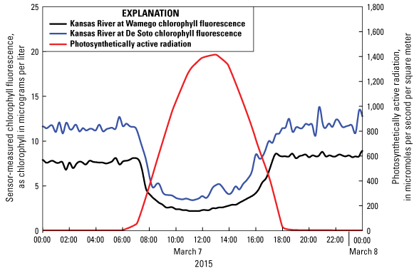
Graph of diurnal variability in sensor-measured chlorophyll fluorescence as chlorophyll in micrograms per liter, during a 24-hour period in March 2015 at the Kansas River at De Soto, Kansas (U.S. Geological Survey Station 06892350) and the Kansas River at Wamego, Kansas (U.S. Geological Survey Station 06887500), compared to photosynthetically active radiation. Fluorescence data are from U.S. Geological Survey (2016c). Hourly surface downwelling shortwave radiation data from the North American Land Data Assimilation System (Xia and others 2012) was converted to photosynthetically active radiation using the coefficients from Britton and Dodd (1976).
Interferences Affecting In-Place Measurements of Algal Pigment Fluorescence
Fluorescence measurements of all types are susceptible to interference from substances that affect how the emitted (excitation) light propagates through the solution, as well as how the fluoresced (emission) light propagates back through the solution to the photodetector. In addition to particle concentration, physical properties such as size and type of particles can affect both absorption and scattering of photons, whereas chemical properties such as DOM and other dissolved constituents primarily affect absorption (fig. 7). Both scattering and absorption, collectively known as “matrix effects” (Pellerin and others, 2013), attenuate light because they result from properties of the matrix in which the fluorescence measurement is being made. Strategies for reducing matrix effects could be necessary in challenging environments. One such strategy that has been applied to other measurement types (nitrate, DOM, and so on) is physically filtering out particles prior to sensor measurements, but filtering cannot be applied to algal fluorescence, because the algal material would be removed by most filters.
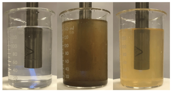
Photographs illustrating conditions affecting the attenuation of fluorescence in water free from particles and solutes (left), in water with particles (center), and in water with colored dissolved organic matter (right). Photographs by Joshua Rosen, U.S. Geological Survey.
Matrix Effects—Scattering and Absorption
The most common sources of interference are scattering and absorption of light by particles and solutes (fig. 8). Scattering by particles in the optical path of the sensor redirects the light outside the measurement area, resulting in lower excitation energy interacting with algae and corresponding lower fluorescent emissions. Further, the emitted fluoresced light is scattered away from the detector, lowering the amount of light returned to the detector. Absorption of light by particles and absorption of light by solutes (most commonly, colored DOM) have the same overall effect, with the excitation energy from the instrument light source and the fluorescence emission both lowered. Ultimately, at high turbidities (where the solution has a high amount of suspended particles) or at high concentrations of colored DOM, or both, interference can be severe enough that the instrument loses sensitivity and does not respond to changes in algal fluorescence.


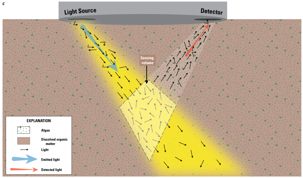
Diagrams showing the effects of scattering and absorption of light on excitation and algal fluorescence emissions in environmental waters. A, Light energy and algal fluorescence emissions in water free from particles and solutes; B, Light energy and algal fluorescence emissions in water with particles; and C, Light energy and algal fluorescence emissions in water with dissolved organic matter.
The effects of particles and DOM attenuation on in-place fluorescence measurements can be substantial and vary between instrument types (Bertone and others, 2018; Bertone and others, 2019). Manufacturers often use optical filters to reduce some of the interferences, but additional corrections, such as those based on concurrent sensor measurements for turbidity and colored DOM proxies, may be needed. Design differences by manufacturer or between instruments from a single manufacturer typically require that sensor-specific data corrections are made. Beyond a certain severity of matrix interferences, however, corrections are not possible because there is insufficient light received by the instrument to make the measurement. As with other compensations and corrections noted in this report, data reporting should be done using appropriate methods and documentation.
Other Interferences
Other potential interferences, such as air bubbles and stray light, can have a substantial effect on optical measurements. However, both these examples are typically alleviated with mechanical solutions, such as wipers and shade caps, and are not addressed in detail in this report. The presence of accessory pigments (for example, chlorophyll b and chlorophyll c) as well as some pigment degradation products (for example, pheophytin, a degradation product of chlorophyll), have similar absorbance spectra and may fluoresce at the same wavelengths as the algal pigment of interest (for example, chla). If accessory pigments or degradation products are present at high concentrations, relations between fluorescence measurements and laboratory-measured concentrations may be relatively poor. Fluorescence sensors may be able to discern differences among groups of pigments, such as chla and PC, but in-place fluorometers cannot differentiate between the different types of chlorophyll. As such, all fluorescent chlorophyll measurements currently (2022) should be reported as “chlorophyll,” not “chla,” unless a relation with laboratory-measured values has been established.
Fluorometer Reporting Units
Many manufacturers produce instruments which report values in quantitative units such as pigment in micrograms per liter, which can be misleading. Instrument reporting values are typically based on empirically derived relations developed by a manufacturer to generate a lookup table between a secondary standard (such as rhodamine WT dye) and healthy cultures of a single type of algae at a specific growth stage. The choice of reference algae used, which can vary substantially from manufacturer to manufacturer, has been shown to have a substantial effect on sensor output because of the difference of fluorescence yield between species (Vincent, 1983; Proctor and Roesler, 2010; Lawrenz and Richardson, 2011). For example, data from Lawrenz and Richardson (2011) show that 20 µg/L chla measured in the laboratory would correspond to sensor-reported estimates ranging from 3.9 to 32.5 µg/L chla based on the phytoplankton species used for their calibration. In addition, many of the taxa used for manufacturers’ default calibrations are small, unicellular forms that are not necessarily common in environmental samples. In environmental waters, sensors are measuring the fluorometric response of pigments contained within diverse communities of algae with various cell sizes, cell wall thicknesses, colors, shapes, and health. Therefore, quantitative sensor readings are suspect without rigorous comparison (validation) against laboratory-measured pigment concentrations and algal community composition.
Another common reporting unit is relative fluorescence units (RFU). RFU is a measure of sensor response based on a percentage of the operating range of the sensor (0–100 percent). While not directly tied to a quantitative value, RFU can be a good primary reporting unit because it is solely reporting sensor response. If required to meet study objectives, it is up to the user to generate a quantitative relation between RFU and the pigment or algal community metric of interest. In many cases, fluorometric data are most valuable when evaluating relative patterns over time, and from this perspective, RFU is most representative of the signal being measured in comparison to other units which are absolute. Additionally, RFU output is typically linear, so a doubling of the reading would generally equate to a doubling of the pigment, assuming all other conditions (temperature, light, and so on) remain constant. However, the RFU measurement will differ between different makes and models of sensors, so the equivalence of an RFU is sensor specific. The RFU data collected by a particular type of sensor may not be directly comparable to the RFU collected by another type of sensor.
In many cases, instruments will allow the reporting of multiple units simultaneously, which could be an ideal approach depending on study objectives. Sensors that report algal pigment fluorescence in RFU and micrograms per liter may also change the equivalence or scale relating RFU to micrograms per liter based on user-applied calibrations in the secondary standard. Thus, applying the same scale factor to convert between reporting units over periods where calibration history is unknown can result in erroneous data reporting in either RFU or micrograms per liter. Whatever method is chosen, it is critical that the users of fluorescence sensors fully understand the limitations and interferences inherent in this type of data, establish realistic expectations, and acknowledge the effect of the reported units on the interpretation of the data.
Instrument Selection
While several commercially available in-place fluorometers may meet the necessary specifications (for example, detection limit, operating range, and resolution) for most freshwater and coastal applications, several additional factors are worth considering when selecting a sensor for algal fluorescence measurements. Practical considerations for sensor selection such as the desired configuration (open face or flow through) and the data-collection platform may be particularly important. For example, users of a multiparameter instrument may want to consider a sensor that integrates with that platform for consistency and ease of use and consider possible interferences (see section “Factors Influencing Observed Fluorescence”) and other potentially important informational data (see section “Ancillary Data”).
Sensor cost is also an important consideration, as the current (2022) generation of commercially available field fluorometers range from about $2,000 to $30,000 based on several factors. For example, integrated wipers, internal dataloggers, and controllers are included with some but not all sensors. Similarly, the choices of housing materials, microprocessors, and the number of LEDs—which may be important considerations in some environments, particularly for long-term deployments in coastal waters—affect the cost of the instruments.
There are numerous single, dual, and multichannel fluorometers available. The instrument selected depends on several considerations, including the following:
-
Data collection objectives.—Consideration must be given to the end goal of sensor deployment, for example, to answer a specific question, to understand overall algal biomass or a specific algal group, or to conduct long-term monitoring.
-
Data quality.—Each sensor make and model differs in accuracy, precision, sensitivity, and resolution. Many times, sensors do not perform as well as advertised. There is an increasing knowledge base within the USGS about algal fluorometers. It is worth spending time learning about the experience others have had with various sensors before making a final decision about what instrument is best for a given application. For new sensors that have not previously been used, careful testing and assessment should be conducted before deployment (for example, Foster and others, 2021; Johnston and others, 2022).
-
Expected range of conditions and algal assemblages.—The instrument selected should be able to provide data across the expected range of environmental conditions. Selected instruments should also target algal biomass or the algal groups of interest or both.
-
Network comparability.—Data comparability is an important factor to consider, especially for long-term monitoring sites, as different sensor makes and models will not produce equivalent data, regardless of calibration. As a first step, the user should check which sensor types are already in use across existing networks and determine if these meet the needs for their local study and monitoring objectives. By using the same sensor that is predominant in other networks, regional and national data comparability are possible, allowing data from the local study site to be placed in a larger context.
-
Calibration procedures.—Different manufacturers will have instrument-specific calibration procedures, as there are no national or international primary standards for consistency. Some sensors require fluorescing dyes for calibrations, and some use solid-state secondary standards, whereas others allow for direct calibrations to environmental samples. The calibration requirements should also be reviewed to ensure that high-quality calibration data can be collected routinely for quality assurance.
-
User friendliness.—Depending on staff experience operating field fluorometers (for example, students or experienced technicians), ease of use could play a key role in maintaining and operating sensors.
-
Infrastructure.—Power and mounting are critical to maintain quality data. Some instruments might have power requirements beyond what a normal USGS streamgaging site can provide and thus must be evaluated before deployments. Light and flow conditions must be evaluated across a range of seasons and conditions to assess possible interferences.
Data Comparability
Not all fluorometers will yield comparable results, even among the same make and model (Roesler and others, 2017). Fluorometric instruments of different designs commonly do not yield identical or equivalent results in the same sampled water or for different algal species and assemblages. Even sensors (of differing make and model) that report measurements in the same units (µg/L, RFU, and so on) and calibrated with the same standards may not yield identical or equivalent results in environmental waters. For example, in a sensor comparison exercise in the San Francisco Estuary, chlorophyll fluorescence response varied considerably among identical probes during a 2-week period (fig. 9; Stumpner and others, 2022).
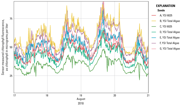
Graph of chlorophyll fluorescence measured by seven fluorometers (five YSI Total Algae-PC sensors mounted on five YSI EXO2 sondes [“YSI Total Algae” on figure] and two YSI 6025 chlorophyll sensors mounted on two YSI 6600 sondes [“YSI 6025” on figure]) in the San Joaquin River at Mossdale, California, between August 17 and August 21, 2018. Figure modified from Stumpner and others (2022).
This variation is because of engineering specifications and the many interferences (chemical, physical, and biological) that are unique to each combination of sensor type and location. Fluorometric sensor measurements are dependent on the optical configuration and the excitation and emission wavelengths of the sensors. This means that the wavelength of light used and the angle and number of detectors used to measure emission response from intracellular pigment molecules all play a role in sensor response. These factors must be well understood when comparing data across sensor networks. When operating field fluorometers, information on sensor type, calibration practices, and so on must all be well documented and available to data users.
Calibration
Approaches for laboratory calibration and checks using standards are described in this section. Primary standards are substances in the purest form that are used to quantify unknown concentrations, including calibrating secondary standards. Secondary standards are standards that have been established by a comparison with a primary standard. Secondary standards include a variety of dyes and solid materials that are relatively inexpensive, stable, and easy to use for verifying sensor operation. Secondary standards composed of variety of materials have been used for algal fluorometers (Earp and others, 2011).
Unlike many other types of sensors, there are no true primary standards for algal field fluorometers, because no standard can be created that will accurately represent the particular mix of algae species (that is, pigment concentrations) and the resultant unique fluorescence response in the environment. Therefore, secondary standards are used for accurate calibration and validation of algal field fluorometers. To do this, the relation between the algal fluorometer unit, a primary standard, and the selected secondary standard must be found. Pure cultures of live algae are used to develop a proxy relation between fluorescence response (the fluorometer unit) under controlled laboratory conditions and extracted pigment concentrations (the primary standard). Fluorescence response and pigment concentrations are then related to a secondary standard (such as rhodamine WT) for calibration.
Laboratory Calibration and Calibration Checks
There is no “truth” when it comes to field fluorometers, at least when “truth” is defined as the real measurement of an extracted pigment concentration or cellular abundance, because fluorescence is a proxy measure based on the fluorescent properties of algal pigments. Even comparison to an extracted pigment sample is only accurate relative to past and future readings if phytoplankton communities and ambient conditions are similar. However, achieving relative comparability in sensors across a network—or in a single sensor over time—is critical for fluorometric datasets. This comparability is achieved through consistent and rigorous calibration practices.
There are many factors that contribute to the frequency and number of calibration checks needed. In general, current (2022) optical sensors like fluorometers should not need to be recalibrated often. However, calibration checks must be made routinely to verify sensor function and verify there is no calibration drift. For continuous deployments, sensors should never go unverified for more than 3 months. Calibration guidance can be found in Anderson (2005) and Hambrook Berkman and Canova (2007) and may be defined in quality assurance plans. For more general information on calibration checks, users should refer to the National Field Manual for the Collection of Water-Quality Data book 9 (U.S. Geological Survey, variously dated), Wagner and others (2006), and the user manual for the instrument.
Calibration checks generally require a two-point check in solutions of known concentration. Deionized water (DIW) is typically used to verify the measurement at zero concentration as the first point, with a secondary standard (rhodamine WT, for example) used to verify another point at a high concentration measurement. A third point could be checked if additional confirmation of linear instrument response is needed. Checks that are within the calibration criteria (table 1) indicate that the instrument is performing as expected. For instruments that fall outside of the calibration criteria, users should ensure that the optical parts are clean and free from staining or scratches, and the measurement is not affected by bubbles, temperature variability, or direct sunlight prior to repeating the calibration check.
In some cases, it may be appropriate to repeat with a separate set of standards, ideally from a previously unopened (or freshly made) bottle, to confirm the readings prior to recalibrating the instrument. Although many dyes are stable for at least a year at room temperature when stored in a dark bottle, it is important to recognize that they will degrade over time (diluted dyes can last only hours to days depending on storage conditions) and will need to be replaced. Users should follow expiration dates and conduct routine laboratory checks if degradation is suspected.
Table 1.
Calibration criteria for algal fluorescence sensors. Percentage is used universally, as there is too much variability in reporting units among manufacturers.[±, plus or minus]
-
• Temperature stability during calibrations.—Standards should be at a stable temperature, as many calibration procedures of different sensor models link the expected reading to a temperature value. More importantly, fluorescence of the standard is temperature dependent. Because standards are sometimes stored in refrigerators, ample time must be allowed for standards to reach room temperature before proceeding.
-
• Cleanliness of all equipment used.—All equipment, from sensors to labware, must be free of contamination prior to their use in calibrations.
-
• Consistent light conditions.—Efforts must be taken to reduce possible interference from external light sources. Use an appropriate calibration vessel or accessories provided by the sensor manufacturer to limit interferences. Calibration vessels made of reflective material which may fluoresce, or leach fluorescing substances, should be avoided. However, calibrations in the laboratory setting are preferred as light conditions are likely to remain stable over time, barring major changes in laboratory lighting (like switching from fluorescent to LED lighting). Consideration must be given to any windows in the laboratory space, and if they should be covered during calibrations.
-
• Conditions conducive to staff being able to focus on calibrations.—Calibrations should not be rushed, or done carelessly, or as a “check the box” exercise. Proper planning to collect the correct materials and allow adequate time (including troubleshooting of potentially erroneous readings) will go a long way to ensure quality, consistent calibrations.
Recalibration of a sensor should only be done when all potentially interfering factors, including those listed above, are confidently eliminated, thereby ensuring that the sensor is in fact out of calibration specifications (table 1). Otherwise, increased possibility of human-induced error, particularly in preparing the secondary reference standard, can be introduced through the erroneous recalibration of instruments. Recalibrating a sensor should not be needed routinely; sensors found out of calibration specifications are more likely indicative of calibration error or sensor failures than calibration drift.
Resetting the calibration of a sensor to the factory default may be needed when calibration error is apparent, and in other rare circumstances. For instance, when the calibration history of the sensor is in question, a factory reset (or “uncal”) can be performed on some sensors according to the guidance in the user manual. Care should be taken when considering whether to reset a sensor, as it may be difficult or impossible to formulate a mathematical correction to apply to data in the current time series collected prior to the factory reset. After resetting the sensor's calibration, verify and recalibrate if necessary.
Secondary Standards
As stated previously, unlike many other types of sensors, there are no true primary standards for algal field fluorometers. The measurement being collected by field fluorometers is the fluorescence response of algal pigments, and not the concentration of algal pigments. A secondary standard can take many forms; however, rhodamine WT dye has been recommended by several manufacturers because of its high solubility in water, known optical properties, and stability over periods of months to years when stored in the dark at room temperature. Rhodamine WT solutions at various concentrations are available through several manufacturers. A two-point calibration conducted with a zero solution (preferably DIW) and a temperature-indexed value from a rhodamine WT secondary standard allows for standardization across sensors.
If users choose to prepare diluted standards from a concentrated stock solution, it should be done using class A volumetric glassware (volumetric flasks, graduated cylinders, or pipettes) under carefully controlled laboratory conditions as described by Wilson and others (1986), and the concentration of the diluted standard should be verified using an independent benchtop or portable instrument. Care is essential when transferring rhodamine WT using pipettes because the viscosity of the solution may result in inaccuracies in volumes mixed. In addition, diluted rhodamine WT mixtures are not as stable and should be used within 5 days of preparation.
Absorption of rhodamine dyes typically ranges between about 440 and 680 nm (Gofman, 1972; Licha and Resch-Genger, 2014; Sugiarto and others, 2017). Measuring absorbance at the peak wavelength (for example, about 556 nm for rhodamine WT) with a spectrophotometer is one way to evaluate rhodamine WT standards to determine the expected absorbance at a given concentration, and thus verify the accuracy of a diluted standard. This is especially true if making rhodamine WT dilutions from concentrate, because error can come about from the operator or the equipment. The ability to verify rhodamine WT standard will depend on the availability of benchtop photospectrometers or fluorometers. Correct benchtop readings of properly diluted rhodamine WT must be determined empirically for any given benchtop instrument. It is important to ensure that benchtop readings are consistent for every batch of rhodamine WT standard, thereby eliminating the standard as a source of calibration error. While this approach to ensuring standard consistency over time is focused on rhodamine WT, the same general approach (that is, determining absorption maxima and measuring every batch of standard made) would apply to any standard created or used.
Alternate Standards
Instrument manufacturers are developing alternative standards, and some now offer options available to users. Solid standards incorporate a piece of solid material that will produce a known fluorescence response. However, the method and material used for alternative standard calibration may not produce equivalent results to those of typical methods and materials. It is up to the end user to follow the manufacturer’ instructions, evaluate new standards, their effects on data quality, and data comparability across sites and data collection networks.
Reference Sensors
Maintaining a field fluorometer for dedicated laboratory use may be a better option for validating the accuracy of diluted standards relative to the sensor output (Alliance for Coastal Technologies, 2017). Such a sensor (sometimes referred to as a reference sensor) is one that has been validated, either by the manufacturer or through internal procedures, and is maintained in the servicing office for no other purpose than for calibrated reference measurements. A well-documented quality assurance plan, like that used to track NIST traceable thermometers, should be maintained to ensure proper functionality of the reference sensor, and provide a traceable calibration history. A reference sensor should be used under the following guidelines:
-
• never take the reference sensor into the field,
-
• never calibrate again after the initial calibration,
-
• always use the reference sensor during calibration checks,
-
• keep a clear, traceable history (for example, similar to methods sometimes used to maintain NIST-traceable thermometers),
-
• routinely check the reference sensor in laboratory-validated secondary reference standard, and
-
• keep the reference sensor safe and secure in a set location when not in use.
Reference sensors are not necessary if you have a benchtop instrument that can verify the accuracy of standards. However, reference sensors are useful to ensure that the standard solutions are consistent so that intercalibration among different sensors in a network can be achieved and validated. For example, standard values outside of ±5 percent of the expected range based on the reference sensor would need to be remade.
Manufacturers’ Instructions
Considering the wide variety of fluorometers on the market, and the inherent differences caused by different manufacturing techniques, components, and styles, it is unlikely that a universal approach to calibrations would be appropriate. Each instrument’s operating manual should be the authoritative reference for calibrating any given fluorometer model. These procedures should be weighed against the requirements of other overarching organizational standard protocols.
Algal Field Fluorometer Use
Algal field fluorometers can be used using several approaches, all of which have relevance based on data collection objectives. Care must be taken to ensure the method chosen meets those objectives, and confounding factors are accounted for appropriately. In each approach, the optical parts of field fluorometers require a high level of care and protection to maintain high-quality measurements over time. Additional guidance on the maintenance and care of field fluorometer optical parts can be found in manufacturer instructions, or general guidance can be found in Wagner and others (2006).
Laboratory Use
In some instances, instruments designed to be used as field fluorometers are maintained in the laboratory, and environmental samples are collected and brought to the laboratory for fluorescence measurements of algal pigments. This approach can reduce environmental influences and interferences on fluorescence measurements, but long holding times between sample collection and measurement could affect the health and viability of algae, thereby affecting fluorescence response. Using field fluorometers in the laboratory for discrete sample measurements should be approached with a full understanding of the effects that discrete sample collection and transport may have on resultant measurements and data interpretation. Data collected using this approach should not be stored under the same parameter code as in-place field measurements, because the approaches are not directly comparable.
Field Use
There are numerous ways algal fluorometers can be used in the field, including continuous fixed site or moored deployments, as a field meter during operation and maintenance of a in-place sensor, for point sample measurements during sample collection, and spatial surveys. Each of these approaches are discussed in more detail below. Additional guidance for field use of algal fluorometers can be found in Hambrook Berkman and Canova (2007) and U.S. Geological Survey (2018c).
Continuous Fixed-Site Monitoring
A key consideration in the deployment of any sensor for continuous monitoring at a fixed site is the identification of a stable, secure location that is representative of the waterbody or location of interest. Guidance on site selection and instrument deployment are provided in Wagner and others (2006), including advice on placement of the instrument within the waterbody, and those guidelines generally apply to the use of fluorescence sensors. There are, however, some features unique to continuously monitoring fluorometers that warrant further attention that are described in this section.
Safety
Standard operating procedures for the safe deployment and operation of continuous monitors and water-quality samplers are always to be followed (for example, Lane and Ray, 1998). It is important that users never look directly into the measurement path of these instruments while they are operating because the intense light can cause immediate injury and permanent damage to the eye. Standard safety precautions, such as grounding rods, lightning arresters, and surge protectors also should be considered when deploying sensitive electronics at monitoring sites.
Physical Infrastructure
As with other water-quality sensors, algal field fluorometers can be deployed either in place or in a pumped configuration external to the waterbody that is being measured. General advantages and disadvantages of in-place and pumped configurations are described in Wagner and others (2006) and Pellerin and others (2013). In addition, instruments located external to a waterbody (for example, in a streamgage) are often accessible under all flow conditions, may experience less biofouling, require shorter distances for power and communication, and allow for the possibility of sampling from multiple locations across the channel with one sensor using multiple intake lines. Disadvantages include increased power requirements for pumps, increased costs, high frequency of site visits to replace tubing, and fouling within the intake lines. Pumps could also result in increased bubbles in the water being sampled, causing erroneous sensor response. Another disadvantage is that if algae are affected in the process of pumping, readings will be different from more direct in-place measurements. Comparisons should be made to fully characterize any differences that might result from measurements of pumped water.
Sensor Mounting
Open-face fluorometers should be mounted vertically with the sensor optical windows oriented downward to avoid the effects of stray light on the optical measurements. This orientation will also limit the accumulation of sediments on the sensor face, but a wiper or other antifouling method is often still necessary to eliminate bubbles and minimize biological fouling. Instruments can be mounted using corrosion-resistant brackets that allow for a secure fit and limit stress to the sensor housing or infrastructure. Hanging the instruments is an alternative approach, but bridles or additional lines may be needed to avoid putting strain directly on sensor cables and connectors. Flow-through configurations may be in any orientation if water is pumped through the sensor at each sampling interval.
Antifouling Measures
Antifouling measures come in two forms: passive chemical guards and mechanical devices (fig. 10). Copper metal accessories, a type of passive chemical guard, are used on a broad range of in-place instruments because of copper’s antibiofouling properties. Options include guards, face plates, copper adhesive tape and mesh screens. In addition, most manufacturers rely on mechanical wipers to keep the optical parts free of sediment, mineral precipitates, and biological growth. Wipers are made of nylon brushes, foam, or silicone blades (fig. 10). Wipers can be integrated into an instrument, or external, add-on components that require separate power and control. Wipers are typically field serviceable and need to be inspected for proper functionality during each site visit and cleaned or replaced per manufacturer recommendations. For sites where copper and wipers are not effective, other antifouling components such as flow-through chambers are also available. When available, the user should record the wiper position along with fluorescence data, in the event the wiper was positioned over the sensor while fluorescence data was collected, to assist in quality assurance and data review as well as troubleshooting. For a comprehensive review of current and future antifouling measures for water quality sensors, see Delgado and others (2021).
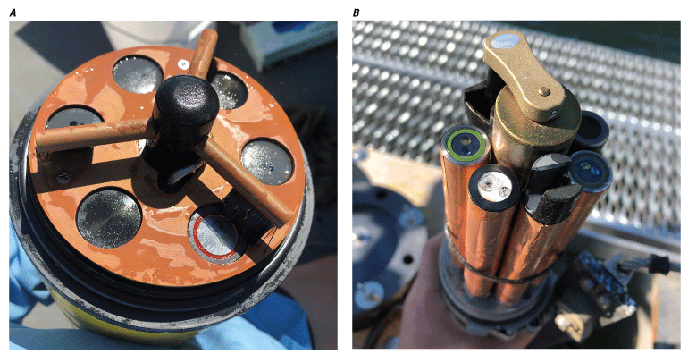
Photographs of anti-fouling measures that may be used with field fluorometers. A, Turner Designs PhytoFind with copper components and integrated wiper; and B, YSI Inc. EXO2 with central wiper and copper tape. Photographs by Sabina Perkins, U.S. Geological Survey.
Dataloggers and Controllers
The current (2022) generation of algal fluorometers use integrated microcontrollers to control excitation and detection, process the incoming signal, and output data to a DCP. Whereas some fluorometers simply provide an output signal that is proportional to the level of fluorescence, others contain an internal clock that enables sample scheduling, biofouling control and internal datalogging. Field fluorometers typically use conventional, industry-standard communication protocols including SDI-12 and RS-232 interfaces, allowing the user to use the instrument with a range of commercially available DCPs. Analog data outputs are often easier to integrate with typical DCPs than digital, but digital output may be preferable if long cable distances are needed or if there are other concerns about signal integrity.
Power and Communication
As connectors and cables are submerged in environmental waters, exposed to harmful effects of ultraviolet light, and subject to oxidation, they can rapidly degrade and affect the transmission of power and data. Cables should be inspected for wear and replaced regularly. Cables can either be purchased from the manufacturer, a third-party vendor, or made to specification, as listed in the sensor manual. A cable made with an outer jacket of polyether or polyurethane is more resistant to wear than standard cable materials and should be used in harsh environments. For instruments with analog output, signal degradation may be an issue if the sensor is further than 10 meters from the DCP. For lengths over 50 meters, users may consider using an instrument with digital communication which aids in preserving signal integrity. For transmitting digital signals by RS-232 over long cable runs, shielded ultralow capacitance cable may be necessary to preserve signal integrity.
Field Meter
An independent field sensor (also referred to as a “field meter”) is used to document changing environmental conditions during servicing and can also serve as a check on the deployed site sensor (Wagner and others, 2006). A field meter can also be used for cross-sectional surveys, vertical profiles, or other measurements that verify the data collected by the site sensor are representative of the area of interest. For algal fluorometers, a sensor of the same design as the site sensor should be used, and measurements made at the same location and elevation as the site sensor for several sampling intervals, following guidelines in Wagner and others (2006). Sensors of different designs from the site sensor should not be used as a field meter, because they may report substantially different values. Local and project quality assurance plans should specify calibration intervals and purposes of field meters based on appropriate USGS policy and technical references. If no other options are available, a different make and model field meter from the site sensor can help indicate large changes in environmental conditions during servicing. When a different make or model from the station sensor must be used, the servicing period should be short, and ideally, environmental change during servicing should be relatively small so that the use of a one-point variable data correction (Wagner and others, 2006, eq. 4) is used. If substantial fouling is indicated while servicing two sensors of different makes or models, deletions of affected data would be favored over fouling corrections because a two-point variable data correction (Wagner and others, 2006, eq. 5) would be inappropriate.
Point Sampling
Algal fluorometers can be used to provide ancillary data for discrete water samples, following the guidelines found in Wilde (variously dated b), or simply as a method to measure algal fluorescence specific locations or depths. As with any field fluorometer use, the resultant data must be assessed for interferences and other confounding factors that affect measurements.
Spatial Surveys
Algal fluorometers have also proven valuable for studies over large areas in rivers, lakes, reservoirs, and estuaries (Downing and others, 2008; Sackmann and others, 2008; Crawford and others, 2015; Foster and others, 2017, 2019; Stumpner and others, 2020). These tend to be short-term studies that evaluate spatial variability in algal biomass or community composition and other physical and chemical parameters (such as temperature and nutrients). Spatial studies generally require that the sample output and sensor equilibration rates are fast enough to measure the variability in water quality during sampling, based on the rate of movement. For example, vertical profiles with a descent rate of 1–10 centimeters (cm) per second require a rapid sampling rate (at least one measurement every few seconds) to be effective at quantifying vertical variability. In addition to the measurement frequency, one must also consider the potential lag time between the exposure of the sensor to a change in conditions and the sensor response. Fortunately, the response time for most algal fluorometers tends to be short (less than 1 second). For a specific study site or application, users should verify the depth limitations of their sensors and consider whether a sensor with a deeper rating is needed. Time of day must also be taken into consideration during planning and data analysis due to the many interferences, such as nonphotochemical quenching, that could affect data.
Ancillary Data
Ancillary data collected concurrently on parameters other than fluorometric response can often allow for additional analysis and interpretation insights. Algae respond to environmental factors like light and temperature and may influence other factors such as pH and dissolved oxygen. These interactions and relationships are sometimes nuanced and complex (fig. 11); however, these parameters should be considered in any data collection activity to meet study objectives and help interpret (or correct if future guidance is established) algal fluorescence data.
Ideally, ancillary data and samples for comparison with algal fluorescence measurements should be collected close to the fluorometer, no matter what approach is being used for deployment. Removing water from the environment to make fluorescence measurements under more controlled conditions (such as a laboratory or darkened bucket) may affect algal fluorescence response and comparisons may not reflect in-place relations.
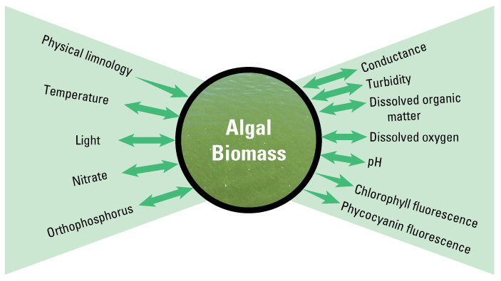
Conceptual diagram of the relations between algal biomass and environmental variables that can currently be measured using in-place sensors. Arrows indicate variables that exert control on algal biomass and variables that are influenced by algal biomass. Actual relations and interactions between environmental variables and algal biomass are more nuanced than indicated in this conceptual diagram.
Ancillary data collection is often dependent on study objectives. Hambrook Berkman and Canova (2007), Graham and others (2008), and U.S. Geological Survey (2018c) describe suggested ancillary data collection for studies focused on algal biomass and community composition in detail. The following are descriptions of several parameters that are recommended for measurement when collecting algal fluorescence data:
-
• Temperature regulates algal growth and has a substantial influence on algal fluorescence response. Collecting temperature data will help inform interpretation of within- and among-site variability in algal fluorescence and may be used to develop site-specific temperature corrections for algal fluorescence data. Some algal fluorometers require temperature for internal data compensation.
-
• Light has a strong influence on algal fluorescence (fig. 6). Collecting light data (using a photosynthetically active radiation [PAR] sensor, for example) will help interpret observed diurnal patterns in algal fluorescence.
-
• Dissolved oxygen concentrations may be influenced by algal activity. Strong diurnal patterns in dissolved oxygen may be indicative of healthy algal populations and can be used to corroborate observed patterns in algal fluorescence (fig. 12).
-
• pH may also be influenced by algal activity. Strong diurnal patterns in pH may be indicative of healthy algal populations and can be used to corroborate observed patterns in algal fluorescence (fig. 12).
-
• Specific conductance may influence algal community composition and health. In some multiparameter instruments, specific conductance data are used for internal compensation of other measurements (for example, dissolved oxygen), and their inclusion should be evaluated with respect to how a particular instrument model performs internal data compensations. Additionally, algae cells have been shown to degrade (or lyse) in higher salinity waters, which would greatly affect the fluorescence response (Rosen and others, 2018).
-
• Turbidity alters the underwater light environment and may interfere with algal fluorescence measurements. Collecting turbidity data will help inform interpretation of within- and among-site variability in algal fluorescence and may be used to develop site-specific turbidity corrections for algal fluorescence data.
-
• Dissolved organic matter also alters the underwater light environment and may interfere with algal fluorescence measurements. Collecting dissolved organic matter data (directly or through proxies like fluorescent dissolved organic matter [fDOM]) will help inform interpretation of within- and among-site variability in algal fluorescence and may be used to develop site-specific dissolved organic matter corrections for algal fluorescence data. Some algal fluorometers apply internal corrections for dissolved organic matter, but often require site-specific discrete sample data for these corrections to work properly.
-
• Algal pigment concentration is measured by proxy with fluorescence measurements. Because fluorescence is what is being measured by algal fluorometers, a quantitative measure of algal pigment concentration can be a valuable quantity to compare with sensor-measured data. These data may also facilitate the development of a proxy relation between algal fluorescence and pigment concentration (fig. 4). However, development of such a relation is not always straightforward because algal cell size, morphology, health, community composition, quenching, and interferences all affect algal fluorescence response (fig. 13).
-
• Algal abundance and community composition data provides the most detailed information on what algae are present, their concentration, and what changes are occurring over time. As noted for algal pigments, proxy relations between these and algal fluorescence may be developed, but the relations are not always straightforward. Shifts in algal community composition may result in substantial changes in algal fluorescence without overall changes in algal abundance (fig. 13).
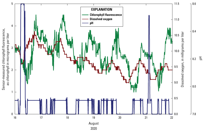
Graph of diurnal variability in chlorophyll fluorescence, dissolved oxygen, and pH during one week in August 2020 in Owasco Lake, New York (U.S. Geological Survey Station 425327076313601). Data are from U.S. Geological Survey (2016c).
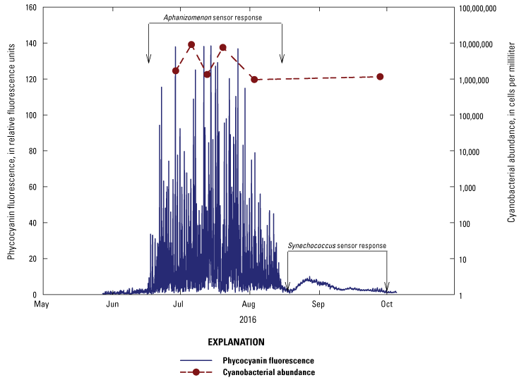
Graph showing phycocyanin fluorescence during a shift in cyanobacterial community composition (but not abundance) in Upper Klamath Lake, Oregon (U.S. Geological Survey Station 422305121553803) during May through October 2016. Phycocyanin fluorescence data are from U.S. Geological Survey (2016c). Cyanobacterial community composition data are from Beauto and Leininger (2021).
Quality Assurance Procedures
Data quality assurance procedures for field fluorescence sensors generally follow USGS methods for continuous water-quality monitors (Wagner and others, 2006). Continuous time-series records first undergo an initial analysis in which erroneous data are flagged or removed from public access. Next, data corrections to account for sensor fouling and calibration drift are applied based on information collected during site visits and during sensor calibration checks. At this point, the corrected dataset reflects the fluorescence that was observed, expressed in terms of the selected output units of a given sensor. These data themselves can be an end product, as long as they are identified as such. Some users may apply additional corrections based on site-specific relations to compensate for temperature effects or interferences from particles and organic matter, as previously discussed. Data corrected in this manner must be stored under different parameter codes and identified as such. Lastly, the data undergo a final evaluation that includes peer review and approval by a technical reviewer with expertise in all processes used to produce the results. Record audits of fluorescence data should follow appropriate organizational policy and guidelines.
All inspection, calibration, ancillary, raw and corrected data are stored in the National Water Information System Time Series (NWIS-TS) database and the USGS Site Information Management System station description (as per Wagner and others, 2006) along with project or site information following project and science center data-management and quality-assurance plans, and continuous records processing policies. Calibration standard operating procedures may be project specific or described as part of a quality assurance plan (particularly if it includes a benchtop photospectrometer to validate rhodamine WT calibration standards). Data corrections are applied as soon as possible after site visits, and data between bookend site visits, are analyzed and approved within the timelines specified by USGS continuous records processing policy (U.S. Geological Survey, 2010, 2017). Results from most algal fluorescence sensors generally are expected to meet the criteria for category 1, although category 2 designation may be appropriate when longer-term laboratory data are needed for record computation or complex water-quality sensors are used that require a longer period of time to develop proficiency. Consistent with that policy, it is reasonable that fluorescence sensor data would be initially classified as category 2, providing additional time (up to 240 days) to characterize site specific confounding effects not otherwise accounted for by the instrument. A category 1 designation (approval within 150 days) may become appropriate once the site conditions are well-understood and field operations become routine. A category 3 designation can be appropriate for highly complex sensor records or for computed time series based on surrogate models. Data assignments to category 2 or 3 are temporary and should be for no more than two years. Associated data that may need to be stored and archived in support of data review include high-frequency burst data, instrument diagnostic data, and laboratory quality-assurance data.
Fouling and Drift Corrections
Corrections for continuous water-quality sensors should be applied when a specified threshold for the sum of the absolute values of the computed fouling and drift corrections are exceeded (table 1; Wagner and others, 2006). Whenever the thresholds are not exceeded (table 1), corrections do not need to be applied. However, users may wish to evaluate instrument accuracy in the laboratory to determine if more stringent, project-specific criteria are justified to meet data quality objectives. If less stringent corrections criteria are applied to a dataset, it should be released in an acceptable digital repository such as ScienceBase (https://www.sciencebase.gov/catalog/) rather than NWIS.
Sensor Fouling
Fouling corrections for field fluorescence sensors account for reductions in transmittance of the excitation or emission light signals from biological growth or sediment accumulation on the sensor optical parts. For most sites and deployment configurations, the sensors can be kept clean using antifouling measures such as wipers and copper components. Fouling corrections may be applied as needed.
Typically, spikes of highly variable data in algal fluorescence datasets are not deleted. Spikes in algal fluorescence data time-series are often a normal result of the presence of various types of algae and can be indicative of algal blooms depending on the algal species present (fig. 13). These spikes provide useful insights into algal activity, and data analysts should resist the urge to delete them subjectively, because they might correspond to a similar spike in a corresponding data time series, such as turbidity. It is important to consider on a site-by-site basis whether a spike in a data time series is erroneous or is an accurate detection of fluorescence. In many cases, ancillary data can assist in the analysis of spikes and provide justification for keeping or deleting them. Developing study-area or project-specific guidelines for identifying erroneous spikes compared to true fluorescence spikes is a recommended best practice.
Data from fluorescence sensors of different make or models are not equivalent. For the best results, a field meter used during servicing of an in-place sensor should be manufactured by the same company that made the in-place sensor. Wagner and others (2006) specifically note that a field meter is used to measure how much environmental conditions are changing during the time a sensor is being serviced and does not show validity of the fluorescence data. As such, a different make and model field meter from the site sensor could indicate changes in environmental conditions during servicing, which could prove useful during record analysis and computation, but those values should not be used to compute data corrections.
Finally, great care must be used while evaluating computed fouling corrections because of the many confounding factors discussed earlier in this document. Differences in readings between the field meter and in-place sensor may not be caused by changes in environmental conditions, but more localized factors like differences in light or suspended particles. Because of this, the use of field meter readings in fouling corrections should be done with caution, and if other water-quality measurements are recorded concurrently, they could provide additional basis to evaluate if conditions meet the criteria for “rapidly changing conditions” as defined by Wagner and others (2006). Equations and guidance for the application of fouling corrections can be found in Wagner and others (2006) and are applicable to algal fluorescence time-series, assuming the guidance in the previous paragraphs is considered in their application.
Calibration Drift
Field fluorescence sensors may have some variation in their response over time, typically because of changes in the performance of their light sources or detectors. However, as noted previously, fluorometer drift is often minimal because of the stability of the solid-state components, and great care should be given to assessing if sensors have drifted, or if check readings out of specifications are because of other factors.
As described previously, calibration drift can be evaluated using the differences in sensor response in at least two standards; DIW used as a zero solution and another of known concentration such as rhodamine WT. The magnitude of the calibration drift error measured in this way allows computations of drift corrections documented by Wagner and others (2006).
Data Reporting
Algal fluorometer data may be reported in a variety of ways, including through the National Water Information System (NWIS) and data releases. Results reported in NWIS must be reported with the parameter and method codes that accurately describe the details of the sensor measurement, which varies depending on the fluorometer, technique, and unit of measurement used. Data reported through other means should include details on the sensor, settings, and specifications that were used during data collection as well as information on any corrections and quality assurance procedures that may have been applied to the data.
Reporting Parameter and Method Codes
There is not one universal NWIS parameter code for algal fluorescence, because there are several different types of algal pigments that can be measured, and measurement units that can be used. The recommended NWIS parameter codes for fluorescence sensor output of the algal pigments most commonly measured by the USGS are described in table 2.
Table 2.
U.S. Geological Survey National Water Information System parameter codes for algal pigments measured by field fluorometers.[The “f” included with all abbreviations designates that data are the result of fluorescence-based measurements. measured by field fluorometers. RFU, relative fluorescence unit; µg/L, microgram per liter]
The “f” included with all abbreviations designates that data are the result of fluorescence-based measurements. If new parameter codes for algal fluorescence data need to be requested, the “f” designation should be used. Parameter codes for other less-commonly measured algal pigments also are available for use in NWIS.
The “estimated from reference material” description included with parameter units other than RFU (RFU is a sensor-specific unit) means that reported concentrations are based on a manufacturer supplied conversion table between a secondary standard (such as rhodamine WT dye) and a primary standard commonly based on a single algal reference culture. If new parameter codes need to be requested for reporting units other than RFU that are based on a manufacturer-supplied conversion, the “estimated from reference material” description should be included.
Method codes are used to identify the equipment used to carry out measurements. NWIS method codes for algal fluorometers most commonly used by the USGS are listed in table 3.
Table 3.
U.S. Geological Survey National Water Information System method codes for commonly used field fluorometers.[nm, nanometer; NA, not applicable]
Method codes for other algal fluorometers also are available in NWIS and can be looked up at https://help.waterdata.usgs.gov/code/method_cd_query?fmt=html. New method codes can be requested for sensors or configurations not currently on this list. Method code requests for new makes and models of algal fluorometers should include information about the following: manufacturer; model; excitation, emission and bandpass wavelengths; and reference organisms used to develop the conversion table between a secondary standard and pigment concentration.
Field Fluorescence to Estimate Quantitative Algal Data
Some users may want to use field fluorescence data as a surrogate for algal pigment concentrations (for example, chla or phycocyanin), algal biomass, or other measures of an algal community. In these cases, empirical or statistical modeling can potentially be used to quantify the relation between algal fluorescence-sensor data and the desired endpoint, typically using results from discrete water-quality sample analyses. Relations must be based on site-specific data. The ability to develop a good relation depends on a variety of factors, such as those previously discussed in the “Factors Influencing Observed Fluorescence” and “Ancillary Data” sections. Flexibility in model development may be required to account for seasonal or long-term changes in the relation between field fluorescence and laboratory measurements because of changes in species composition or other factors influencing algal fluorescence response. There are several methods (regression analysis, for example) that can potentially be used to achieve model-derived computations of pigment concentrations or algal abundance in the waterbody (Roesler and others, 2017), however the techniques, methods, and reporting policy for such efforts are beyond the scope of this report. Similarly, any published time-series regression or other model that relies on discrete samples should maintain some level of sampling effort if publication of the computed result is to continue.
Computed pigment concentration or algal abundance based on fluorescence may be stored in NWIS but must be entered under a parameter code that clearly indicates the concentrations are indirect estimates. In addition, the model used to compute concentrations must be appropriately documented and published. Available NWIS parameter codes for estimated concentrations of algal pigments are listed in table 4.
Table 4.
U.S. Geological Survey National Water Information System parameter codes for common model-estimated algal pigments.[ug/L, microgram per liter; cells/mL, cells per milliliter]
Summary
Many water-quality programs collect fluorescence data related to algal pigments using field-based sensors. Algal pigment fluorescence sensors require a greater understanding of sensor design, environmental interferences, algal dynamics, and limitations than many other sensors routinely deployed by the U.S. Geological Survey (USGS). Algal fluorescence sensors do not directly measure algal abundance, biomass, or pigment concentration, but rather the fluorescence response of algal pigments. The magnitude of fluorescence response can often, but not always, be related to algal pigment concentration. Fluorescence sensors can provide valuable insights into algal biomass and dynamics through relative patterns, and in some cases may be used as indicators of algal blooms. Effective and consistent deployment requires thorough planning and setting realistic expectations for sensor performance and data objectives.
Algal fluorometers have advanced substantially since previous USGS guidance documents were published. This report supplements existing USGS guidance by providing information specific to the principles, selection, and use of field fluorescence sensors for in-place determination of the presence, relative abundance, and qualitative estimates of algal pigment concentrations in environmental waters. Guidance is provided for instrument preparation and deployment, ongoing maintenance and field operations, quality-assurance procedures, and data reporting. Adherence to the guidelines included in this report will help USGS personnel and others collect field data by using algal fluorometers in ways that are consistent and comparable across different studies, sites, and instruments.
References Cited
Alliance for Coastal Technologies, 2017, Sensors for monitoring of harmful algae, cyanobacteria, and their toxins—Alliance for Coastal Technologies Workshop Proceedings, Moss Landing, Calif., January 30–February 1, 2017: Alliance for Coastal Technologies, reference number [UMCES] CBL 2017-026, report number ACT WS01-17, 36 p. [Also available at https://www.act-us.info/workshops.php.]
Alliance for Coastal Technologies, 2019a, Performance verification statement for BBE Moldaenke’s PhycoProbe: Alliance for Coastal Technologies, reference number [UMCES] CBL 2019-006, report number ACT VS19-01, 71 p. [Also available at https://www.act-us.info/evaluations.php.]
Alliance for Coastal Technologies, 2019b, Performance verification statement for Turner Designs CyanoFluor: Alliance for Coastal Technologies, reference number [UMCES] CBL 2019-007, report number ACT VS19-02, 62 p. [Also available at https://www.act-us.info/evaluations.php.]
Alliance for Coastal Technologies, 2019c, Performance verification statement for Turner Designs PhytoFind: Alliance for Coastal Technologies, reference number [UMCES] CBL 2019-008, report number ACT VS19-03, 68 p. [Also available at https://www.act-us.info/evaluations.php.]
Alliance for Coastal Technologies, 2019d, Performance verification statement for JFE Advantech’s multi-excitation chlorophyll fluorometer: Alliance for Coastal Technologies, reference number [UMCES] CBL 2019-009, report number ACT VS19-04, 70 p. [Also available at https://www.act-us.info/evaluations.php.]
Anderson, C.W., 2005, Turbidity (ver. 2.1): U.S. Geological Survey Techniques of Water-Resources Investigations, book 9, chap. A6.7, 55 p., accessed January 27, 2022, at https://doi.org/10.3133/twri09A6.7. [Supersedes version 2.0, released in 1998.]
Beauto, K.V., and Leininger, Z.J., 2021, Phytoplankton data for Upper Klamath Lake, Oregon, 2010–2018: U.S. Geological Survey data release, accessed April 22, 2022, at https://doi.org/10.5066/P9D9BC7R.
Berman, T., 1972, Profiles of chlorophyll concentration by in vivo fluorescence—Some limnological applications: Limnology and Oceanography, v. 17, no. 4, p. 616–618, accessed August 29, 2014, at https://doi.org/10.4319/lo.1972.17.4.0616.
Bertone, E., Burford, M.A., and Hamilton, D.P., 2018, Fluorescence probes for real-time remote cyanobacteria monitoring—A review of challenges and opportunities: Water Research, v. 141, p. 152–162, accessed February 19, 2019, at https://doi.org/10.1016/j.watres.2018.05.001.
Bertone, E., Chuang, A., Burford, M.A., and Hamilton, D.P., 2019, In situ fluorescence monitoring of cyanobacteria—Laboratory-based quantification of species-specific measurement accuracy: Harmful Algae, v. 87, article number 101625, 14 p., accessed July 25, 2019, at https://doi.org/10.1016/j.hal.2019.101625.
Beutler, M., Wiltshire, K.H., Meyer, B., Moldaenke, C., Lüring, C., Meyerhöfer, M., Hansen, U.-P., and Dau, H., 2002, A fluorometric method for the differentiation of algal populations in vivo and in situ: Photosynthesis Research, v. 72, no. 1, p. 39–53, accessed September 11, 2014, at https://doi.org/10.1023/A:1016026607048.
Biermann, L., Guinet, C., Bester, M., Brierley, A., and Boehme, L., 2015, An alternative method for correcting fluorescence quenching: Ocean Science, v. 11, no. 1, p. 83–91, accessed February 22, 2019, at https://doi.org/10.5194/os-11-83-2015.
Britton, C.M., and Dodd, J.D., 1976, Relationships of photosynthetically active radiation and shortwave irradiance: Agricultural Meteorology, v. 17, no. 1, p. 1–7, accessed June 30, 2022, at https://doi.org/10.1016/0002-1571(76)90080-7.
Catherine, A., Escoffier, N., Belhocine, A., Nasri, A.B., Hamlaoui, S., Yéprémian, C., Bernard, C., and Troussellier, M., 2012, On the use of the FluoroProbe, a phytoplankton quantification method based on fluorescence excitation spectra for large-scale surveys of lakes and reservoirs: Water Research, v. 46, no. 6, p. 1771–1784, accessed March 22, 2019, at https://doi.org/10.1016/j.watres.2011.12.056.
Coble, P.G., Lead, J., Baker, A., Reynolds, D.M., and Spencer, R.G.M., eds., 2014, Aquatic organic matter fluorescence: New York, Cambridge University Press, 375 p. [Also available at https://doi.org/10.1017/CBO9781139045452.]
Crawford, J.T., Loken, L.C., Casson, N.J., Smith, C., Stone, A.G., and Winslow, L.A., 2015, High-speed limnology—Using advanced sensors to investigate spatial variability in biogeochemistry and hydrology: Environmental Science & Technology, v. 49, no. 1, p. 442–450, accessed May 8, 2017, at https://doi.org/10.1021/es504773x.
Delgado, A., Briciu-Burghina, C., and Regan, F., 2021, Antifouling strategies for sensors used in water monitoring—Review and future perspectives: Sensors, v. 21, no. 2, article no. 389, 25 p, accessed June 1, 2022, at https://doi.org/10.3390/s21020389.
Downing, B.D., Bergamaschi, B.A., Evans, D.G., and Boss, E., 2008, Assessing contribution of DOC from sediments to a drinking-water reservoir using optical profiling: Lake and Reservoir Management, v. 24, no. 4, p. 381–391, accessed January 14, 2014, at https://doi.org/10.1080/07438140809354848.
Earp, A., Hanson, C.E., Ralph, P.J., Brando, V.E., Allen, S., Baird, M., Clementson, L., Daniel, P., Dekker, A.G., Fearns, P.R.C.S., Parslow, J., Strutton, P.G., Thompson, P.A., Underwood, M., Weeks, S., and Doblin, M.A., 2011, Review of fluorescence standards for calibration of in situ fluorometers—Recommendations applied in coastal and ocean observing programs: Optics Express, v. 19, no. 27, p. 26,768–26,782, accessed July 11, 2014, at https://doi.org/10.1364/OE.19.026768.
Falkowski, P., and Kiefer, D.A., 1985, Chlorophyll a fluorescence in phytoplankton—Relationship to photosynthesis and biomass: Journal of Plankton Research, v. 7, no. 5, p. 715–731, accessed September 11, 2014, at https://doi.org/10.1093/plankt/7.5.715.
Fee, E.J., 1976, The vertical and seasonal distribution of chlorophyll in lakes of the Experimental Lakes Area, northwestern Ontario—Implications for primary production estimates: Limnology and Oceanography, v. 21, no. 6, p. 767–783, accessed January 26, 2018, at https://doi.org/10.4319/lo.1976.21.6.0767.
Foster, G.M., Graham, J.L., and King, L.R., 2019, Spatial and temporal variability of harmful algal blooms in Milford Lake, Kansas, May through November 2016: U.S. Geological Survey Scientific Investigations Report 2018–5166, 36 p. [Also available at https://doi.org/10.3133/sir20185166.]
Foster, G.M., Graham, J.L., Stiles, T.C., Boyer, M.G., King, L.R., and Loftin, K.A., 2017, Spatial variability of harmful algal blooms in Milford Lake, Kansas, July and August 2015: U.S. Geological Survey Scientific Investigations Report 2016–5168, 45 p. [Also available at https://doi.org/10.3133/sir20165168.]
Foster, G.M., King, L.R., Jastram, J.D., Joiner, J.K., Pellerin, B.A., Graham, J.L., and Williams, T.J., 2021, Technical note–Relative variability of selected turbidity standards and sensors in use by the U.S. Geological Survey: U.S. Geological Survey Open-File Report 2021–1009, 41 p., 23 app. [Also available at https://doi.org/10.3133/ofr20211009.]
Gofman, A., 1972, Absorption and fluorescence spectra of rhodamine dyes: Journal of Applied Spectroscopy, v. 17, no. 6, p. 1645–1647. [Also available at https://doi.org/10.1007/BF00618979.]
Graham, J.L., Loftin, K.A., Ziegler, A.C., and Meyer, M.T., 2008, Cyanobacteria in lakes and reservoirs—Toxin and taste-and-odor sampling guidelines: U.S. Geological Survey Techniques of Water-Resources Investigations, book 9, chap. A7.5, 61 p., accessed June 6, 2016, at https://doi.org/10.3133/twri09A7.5.
Gregor, J., and Maršálek, B., 2004, Freshwater phytoplankton quantification by chlorophyll a—A comparative study of in vitro, in vivo, and in situ methods: Water Research, v. 38, no. 3, p. 517–522, accessed August 29, 2014, at https://doi.org/10.1016/j.watres.2003.10.033.
Hambrook Berkman, J.A., and Canova, M.G., 2007, Algal biomass indicators: U.S. Geological Survey Techniques of Water-Resources Investigations, book 9, chap. A7.4, 82 p., accessed June 6, 2016, at https://doi.org/10.3133/twri09A7.4.
Holligan, P.M., and Harbour, D.S., 1977, The vertical distribution and succession of phytoplankton in the western English Channel in 1975 and 1976: Journal of the Marine Biological Association of the United Kingdom, v. 57, no. 4, p. 1075–1093, accessed April 16, 2018, at https://doi.org/10.1017/S002531540002614X.
Johnston, B.D., Graham, J.L., Foster, G.M., and Downing, B.D., 2022, Technical note—Performance evaluation of the PhytoFind, an in-place phytoplankton classification tool: U.S. Geological Survey Open-File Report 2022–5103, 36 p., https://doi.org/10.3133/sir20225103.
Kasinak, J.-M.E., Holt, B.M., Chislock, M.F., and Wilson, A.E., 2015, Benchtop fluorometry of phycocyanin as a rapid approach for estimating cyanobacterial biovolume: Journal of Plankton Research, v. 37, no. 1, p. 248–257, accessed April 16, 2018, at https://doi.org/10.1093/plankt/fbu096.
Lakowicz, J.R., 2006, Principles of fluorescence spectroscopy (3rd ed.): Boston, Mass., Springer, 954 p. [Also available at https://doi.org/10.1007/978-0-387-46312-4.]
Lane, S.L., and Ray, R.G., 1998, Safety in field activities: U.S. Geological Survey Techniques of Water-Resources Investigations, book 9, chap. A9, 75 p., accessed October 1, 2012, at https://doi.org/10.3133/twri09A9.
Lawrenz, E., and Richardson, T.L., 2011, How does the species used for calibration affect chlorophyll a measurements by in situ fluorometry?: Estuaries and Coasts, v. 34, no. 4, p. 872–883, accessed August 29, 2014, at https://doi.org/10.1007/s12237-010-9346-6.
Licha, K., and Resch-Genger, U., 2014, Fluorescent reporters and optical probes, Fluorescent reporters and optical probes, chap. 4.08 of Alves, F., and Keissling, F., eds, Volume 4—Optical molecular imaging, v. 4 of Brahme, A., ed., Comprehensive biomedical physics: Amsterdam, Elsevier B.V., p. 85–109. [Also available at https://doi.org/10.1016/B978-0-444-53632-7.00402-0.]
Lombard, F., Boss, E., Waite, A.M., Vogt, M., Uitz, J., Stemmann, L., Sosik, H.M., Schulz, J., Romagnan, J.-B., Picheral, M., Pearlman, J., Ohman, M.D., Niehoff, B., Möller, K.O., Miloslavich, P., Lara-Lpez, A., Kudela, R., Lopes, R.M., Kiko, R., Karp-Boss, L., Jaffe, J.S., Iversen, M.H., Irisson, J.-O., Fennel, K., Hauss, H., Guidi, L., Gorsky, G., Giering, S.L.C., Gaube, P., Gallager, S., Dubelaar, G., Cowen, R.K., Carlotti, F., Briseño-Avena, C., Berline, L., Benoit-Bird, K., Bax, N., Batten, S., Ayata, S.D., Artigas, L.F., and Appeltans, W., 2019, Globally consistent quantitative observations of planktonic ecosystems: Frontiers in Marine Science, v. 6, article 196, 21 p., accessed February 22, 2021, at https://doi.org/10.3389/fmars.2019.00196.
Lorenzen, C.J., 1966, A method for the continuous measurement of in vivo chlorophyll concentration: Deep-Sea Research and Oceanographic Abstracts, v. 13, no. 2, p. 223–227, accessed August 29, 2014, at https://doi.org/10.1016/0011-7471(66)91102-8.
Maxwell, K., and Johnson, G.N., 2000, Chlorophyll fluorescence—A practical guide: Journal of Experimental Botany, v. 51, no. 345, p. 659–668, accessed February 22, 2021, at https://doi.org/10.1093/jexbot/51.345.659.
Olaizola, M., La Roche, J., Kolber, Z., and Falkowski, P.G., 1994, Non-photochemical fluorescence quenching and the diadinoxanthin cycle in a marine diatom: Photosynthesis Research, v. 41, no. 2, p. 357–370, accessed June 14, 2021, at https://doi.org/10.1007/BF00019413.
Pellerin, B.A., Bergamaschi, B.A., Downing, B.D., Saraceno, J.F., Garrett, J.D., and Olsen, L.D., 2013, Optical techniques for the determination of nitrate in environmental waters—Guidelines for instrument selection, operation, deployment, quality assurance, and data reporting: U.S. Geological Survey Techniques and Methods 1–D5, 37 p., accessed January 14, 2014, at https://doi.org/10.3133/tm1D5.
Proctor, C.W., and Roesler, C.S., 2010, New insights on obtaining phytoplankton concentration and composition from in situ multispectral chlorophyll fluorescence: Limnology and Oceanography: Methods, v. 8, no. 12, p. 695–708, accessed April 4, 2012, at https://doi.org/10.4319/lom.2010.8.0695.
Roesler, C.S., and Barnard, A.H., 2013, Optical proxy for phytoplankton biomass in the absence of photophysiology—Rethinking the absorption line height: Methods in Oceanography, v. 7, p. 79–94, accessed August 19, 2014, at https://doi.org/10.1016/j.mio.2013.12.003.
Roesler, C., Uitz, J., Claustre, H., Boss, E., Xing, X., Organelli, E., Briggs, N., Bricaud, A., Schmechtig, C., Poteau, A., D’Ortenzio, F., Ras, J., Drapeau, S., Haëntjens, N., and Barbieux, M., 2017, Recommendations for obtaining unbiased chlorophyll estimates from in situ chlorophyll fluorometers—A global analysis of WET Labs ECO sensors: Limnology and Oceanography: Methods, v. 15, no. 6, p. 572–585, accessed February 19, 2019, at https://doi.org/10.1002/lom3.10185.
Rosen, B.H., Loftin, K.A., Graham, J.L., Stahlhut, K.N., Riley, J.M., Johnston, B.D., and Senegal, S., 2018, Understanding the effect of salinity tolerance on cyanobacteria associated with a harmful algal bloom in Lake Okeechobee, Florida: U.S. Geological Survey Scientific Investigations Report 2018–5092, 32 p. [Also available at https://doi.org/10.3133/sir20185092].
Sackmann, B.S., Perry, M.J., and Eriksen, C.C., 2008, Seaglider observations of variability in daytime fluorescence quenching of chlorophyll-a in Northeastern Pacific coastal waters: Biogeosciences Discussions, v. 5, p. 2839–2865, preprint posted July 9, 2008, accessed July 17, 2012, at https://doi.org/10.5194/bgd-5-2839-2008.
Smith, S., 2020, What is rhodamine? Get the rho down (updated November 2021): YSI Incorporated web page, accessed May 18, 2022, at https://www.ysi.com/ysi-blog/water-blogged-blog/2020/04/what-is-rhodamine-get-the-rho-down.
Stauffer, B.A., Bowers, H.A., Buckley, E., Davis, T.W., Johengen, T.H., Kudela, R., McManus, M.A., Purcell, H., Smith, G.J., Vander Woude, A.J., and Tamburri, M.N., 2019, Considerations in harmful algal bloom research and monitoring—Perspectives from a consensus-building workshop and technology testing: Frontiers in Marine Science, v. 6, article 399, 18 p., accessed January 6, 2021, at https://doi.org/10.3389/fmars.2019.00399.
Stokes, G.G., 1852, On the change of refrangibility of light: Philosophical Transactions of the Royal Society of London, v. 142, p. 463–562, accessed July 29, 2014, at https://doi.org/10.1098/rstl.1852.0022.
Stumpner, E.B., Bergamaschi, B.A., Kraus, T.E.C., Parker, A.E., Wilkerson, F.P., Downing, B.D., Dugdale, R.C., Murrell, M.C., Carpenter, K.D., Orlando, J.L., and Kendall, C., 2020, Spatial variability of phytoplankton in a shallow tidal freshwater system reveals complex controls on abundance and community structure: Science of the Total Environment, v. 700, article 134392, 17 p., accessed February 22, 2021, at https://doi.org/10.1016/j.scitotenv.2019.134392.
Stumpner, E.B., Yin, J., Heberger, M., Wu, J., Wong, A., and Saraceno, J.F., 2022, San Francisco estuary chlorophyll sensor and sample analysis intercomparison: San Francisco Estuary Institute, SFEI contribution number 977, 61 p., accessed April 22, 2022 at https://deltarmp.org/Documents/Chl%20Intercomparison%20Report_USGS_approval_121521.pdf.
Suggett, D.J., Prášil, O., and Borowitzka, M.A., eds., 2010, Chlorophyll a fluorescence in aquatic sciences—Methods and applications, v. 4 of Borowitzka, M.A., Developments in applied phycology: Dordrecht, Netherlands, Springer, 323 p. [Also available at https://doi.org/10.1007/978-90-481-9268-7.]
Sugiarto, I.T., Isnaeni, and Putri, K.Y., 2017, Analysis of dual peak emission from Rhodamine G6 organic dyes using photoluminescence: Journal of Physics: Conference Series, v. 817, article no. 012047, accessed June 1, 2022, at https://doi.org/10.1088/1742-6596/817/1/012047.
U.S. Geological Survey, [variously dated], National field manual for the collection of water-quality data: U.S. Geological Survey Techniques and Methods, book 9, accessed January 28, 2022, at https://www.usgs.gov/mission-areas/water-resources/science/national-field-manual-collection-water-quality-data-nfm.
U.S. Geological Survey, 2006, Collection of water samples (ver. 2.0): U.S. Geological Survey Techniques of Water-Resources Investigations, book 9, chap. A4, 166 p., accessed January 27, 2022, at https://doi.org/10.3133/twri09A4. [Supersedes version 1.0, released in 1999.]
U.S. Geological Survey, 2010, WMA2010.02 WRD policy numbered memorandum no. 2010.02 continuous records processing of all water time series data: U.S. Geological Survey policy memorandum WMA.2010.02, accessed March 17, 2015, at https://water.usgs.gov/water-resources/memos/memo.php?id=3306.
U.S. Geological Survey, 2011, 502.2–Fundamental science practices—Planning and conducting data collection and research: U.S Geological Survey web page, accessed March 29, 2021, at https://www.usgs.gov/about/organization/science-support/survey-manual/5022-fundamental-science-practices-planning-and. [Supersedes the previous version, released in 2006.]
U.S. Geological Survey, 2016a, 502.3—Fundamental science practices—Peer review: U.S. Geological Survey web page, accessed March 29, 2021, at https://www.usgs.gov/about/organization/science-support/survey-manual/5023-fundamental-science-practices-peer-review. [Supersedes the previous version, released in 2011.]
U.S. Geological Survey, 2016b, 502.4—Fundamental science practices—Review, approval, and release of information products: U.S. Geological Survey web page, accessed March 29, 2021, at https://www.usgs.gov/about/organization/science-support/survey-manual/5024-fundamental-science-practices-review-approval. [Supersedes the previous version, released in 2011.]
U.S. Geological Survey, 2016c, USGS water data for the Nation: U.S. Geological Survey National Water Information System database, accessed September 9, 2021, at https://doi.org/10.5066/F7P55KJN.
U.S. Geological Survey, 2017, GW2017.01, SW2017.05, WQ2017.02 clarification of Water Mission Area policy on continuous records processing of time series data—Categorization of groundwater, surface water, and water quality sites/records: U.S. Geological Survey technical memorandum GW.2017.02, accessed March 23, 2021, at https://water.usgs.gov/water-resources/memos/memo.php?id=452.
U.S. Geological Survey, 2018a, 502.1—Fundamental science practices—Foundation policy: U.S. Geological Survey web page, accessed March 29, 2021, at https://www.usgs.gov/about/organization/science-support/survey-manual/5021-fundamental-science-practices-foundation. [Supersedes the previous version, released in 2011.]
U.S. Geological Survey, 2018b, IM OSQI 2018-01, quality management system for USGS laboratories: U.S. Geological Survey instructional memorandum IM OSQI 2018-01, accessed March 23, 2021, at https://www.usgs.gov/about/organization/science-support/survey-manual/im-osqi-2018-01-quality-management-system-usgs.
U.S. Geological Survey, 2018c, Lakes and reservoirs—Guidelines for study design and sampling: U.S. Geological Survey Techniques and Methods, book 9, chap. A10, 48 p., accessed February 22, 2021, at https://doi.org/10.3133/tm9A10. [Supersedes U.S. Geological Survey Techniques of Water-Resources Investigations, book 9, chap. A10, released in 2015.]
U.S. Geological Survey, 2018d, Preparations for water sampling: U.S. Geological Survey Techniques and Methods, book 9, chap. A1, 42 p., accessed January 27, 2022, at https://doi.org/10.3133/tm9A1. [Supersedes U.S. Geological Survey Techniques of Water-Resources Investigations, book 9, chap. A1, version 2.0, released in 2005.]
Vincent, W.F., 1983, Fluorescence properties of the freshwater phytoplankton—Three algal classes compared: British Phycological Journal, v. 18, no. 1, p. 5–21, accessed September 11, 2014, at https://doi.org/10.1080/00071618300650021.
Wagner, R.J., Boulger, R.W., Jr., Oblinger, C.J., and Smith, B.A., 2006, Guidelines and standard procedures for continuous water-quality monitors—Station operation, record computation, and data reporting: U.S. Geological Survey Techniques and Methods book 1, chap. D3, 51 p. plus 8 attachments, accessed August 6, 2012, at https://doi.org/10.3133/tm1D3. [Supersedes U.S. Geological Survey Water-Resources Investigations Report 2000–4252, released in 2000.]
Watras, C.J., Morrison, K.A., Rubsam, J.L., Hanson, P.C., Watras, A.J., LaLiberte, G.D., and Milewski, P., 2017, A temperature compensation method for chlorophyll and phycocyanin fluorescence sensors in freshwater: Limnology and Oceanography: Methods, v. 15, no. 7, p. 642–652, accessed February 19, 2019, at https://doi.org/10.1002/lom3.10188.
Wilde, F.D., ed., [variously dated] a, Biological indicators: U.S. Geological Survey Techniques of Water-Resources Investigations, book 9, chap. A7, [variously paginated], accessed January 27, 2022, at https://www.usgs.gov/mission-areas/water-resources/science/national-field-manual-collection-water-quality-data-nfm#overview.
Wilde, F.D., ed., [variously dated] b, Field measurements: U.S. Geological Survey Techniques of Water-Resources Investigations, book 9, chap. A6, [variously paginated], accessed January 27, 2022, at https://www.usgs.gov/mission-areas/water-resources/science/national-field-manual-collection-water-quality-data-nfm#overview.
Wilde, F.D., ed., [variously dated] c, Processing of water samples: U.S. Geological Survey Techniques of Water-Resources Investigations, book 9, chap. A5, [variously paginated], accessed January 27, 2022, at https://www.usgs.gov/mission-areas/water-resources/science/national-field-manual-collection-water-quality-data-nfm#overview.
Wilde, F.D., ed., 2004, Cleaning of equipment for water sampling (ver. 2.0): U.S. Geological Survey Techniques of Water-Resources Investigations, book 9, chap. A3, 68 p., accessed January 27, 2022, at https://doi.org/10.3133/twri09A3. [Supersedes version 1.2, released in 2003.]
Wilde, F.D., Sandstrom, M.W., and Skrobialowski, S.C., 2014, Selection of equipment for water sampling (ver 3.1): U.S. Geological Survey Techniques of Water-Resources Investigations, book 9, chap. A2, 78 p., accessed January 27, 2022, at https://doi.org/10.3133/twri09A2. [Supersedes version 2.0, released in 2003.]
Wilson, J.F., Cobb, E.D., and Kilpatrick, F.A., 1986, Fluorometric procedures for dye tracing: U.S. Geological Survey Techniques of Water-Resources Investigations, book 3, chap. A12, 34 p., accessed December 23, 2014, at https://doi.org/10.3133/twri03A12. [Supersedes U.S. Geological Survey Open-File Report 84–234, released in 1984.]
Xia, Y., Mitchell, K., Ek, M., Sheffield, J., Cosgrove, B., Wood, E., Luo, L., Alonge, C., Wei, H., Meng, J., Livneh, B., Lettenmaier, D., Koren, V., Duan, Q., Mo, K., Fan, Y., and Mocko, D., 2012, Continental-scale water and energy flux analysis and validation for the North American Land Data Assimilation System project phase 2 (NLDAS-2)—1. Intercomparison and application of model products: Journal of Geophysical Research, v. 117, D3, article no. D03109, 27 p., accessed June 30, 2022, at https://doi.org/10.1029/2011JD016048.
Conversion Factors
Supplemental Information
Concentrations of chemical constituents in water are given in either milligrams per liter (mg/L) or micrograms per liter (µg/L).
Cycles per second are given in hertz (Hz).
Photosynthetically active radiation is given in micromoles per second per square meter ([µmol/s]/m2).
Abundance of cyanobacteria is given in cells per milliliter (cells/mL).
Fluorescence is given in relative fluorescence units (RFU).
Turbidity is given in formazin nephalometric units (FNU).
Abbreviations
chla
chlorophyll a
DCP
data-collection platform
DIW
deionized water
DOM
dissolved organic matter
fDOM
fluorescent dissolved organic matter
LED
light-emitting diode
NIST
National Institute of Standards and Technology
NWIS
National Water Information System
NWIS-TS
National Water Information System Time Series
OWQ
Office of Water Quality
QMS
Quality Management System
PC
phycocyanin
PE
phycoerythrin
RFU
relative fluorescence units
USGS
U.S. Geological Survey
WMA
Water Mission Area
For more information about this report, contact:
Director, New York Water Science Center
U.S. Geological Survey
425 Jordan Road
Troy, NY 12180–8349
dc_ny@usgs.gov
or visit our website at
https://www.usgs.gov/centers/ny-water
Publishing support provided by the Pembroke Publishing Service Center
Disclaimers
Any use of trade, firm, or product names is for descriptive purposes only and does not imply endorsement by the U.S. Government.
Although this information product, for the most part, is in the public domain, it also may contain copyrighted materials as noted in the text. Permission to reproduce copyrighted items must be secured from the copyright owner.
Suggested Citation
Foster, G.M., Graham, J.L., Bergamaschi, B.A., Carpenter, K.D., Downing, B.D., Pellerin, B.A., Rounds, S.A., and Saraceno, J.F., 2022, Field techniques for the determination of algal pigment fluorescence in environmental waters—Principles and guidelines for instrument and sensor selection, operation, quality assurance, and data reporting: U.S. Geological Survey Techniques and Methods, book 1, chap. D10, 34 p., https://doi.org/10.3133/tm1D10.
ISSN: 2328-7055 (online)
| Publication type | Report |
|---|---|
| Publication Subtype | USGS Numbered Series |
| Title | Field techniques for the determination of algal pigment fluorescence in environmental waters—Principles and guidelines for instrument and sensor selection, operation, quality assurance, and data reporting |
| Series title | Techniques and Methods |
| Series number | 1-D10 |
| DOI | 10.3133/tm1D10 |
| Publication Date | December 27, 2022 |
| Year Published | 2022 |
| Language | English |
| Publisher | U.S. Geological Survey |
| Publisher location | Reston, VA |
| Contributing office(s) | California Water Science Center, Kansas Water Science Center, New York Water Science Center, Oregon Water Science Center, WMA - Observing Systems Division |
| Description | vi, 34 p. |
| Larger Work Type | Report |
| Larger Work Subtype | USGS Numbered Series |
| Larger Work Title | Section D: Water quality in Book 1: Collection of water data by direct measurement |
| Public Comments | This report is Chapter 10 of Section D: Water quality in Book 1: Collection of water data by direct measurement. |
| Online Only (Y/N) | Y |
| Additional Online Files (Y/N) | N |