
Figure 4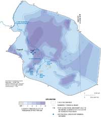
Lateral model boundaries, perennial reaches, confined areas, and initial transmissivity used in simulations of effects of withdrawals in the Leupp, Arizona, area.
Figure 5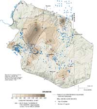
Thickness of the C aquifer, northeastern Arizona, as derived from a hydrogeologic framework model.
Figure 6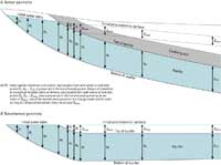
Vertical section of a hypothetical partially confined aquifer. A, Actual geometry. B, Transformed geometry for use in a change model.
Figure 7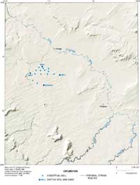
Locations of existing and conceptual wells used in model simulation scenarios A and B for the C aquifer, northeastern Arizona..
Figure 8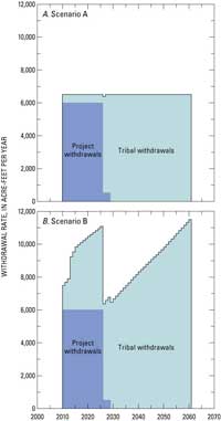
Withdrawal scenarios for model simulations of changes in the C aquifer, northeastern Arizona..
Summary of Numerical Ground-Water Change Model
The numerical code used to simulate changes in water levels in the C aquifer and ground water flow at the head-dependant boundaries is the Modular Three-Dimensional Finite Difference Ground-Water Flow Model (MODFLOW-2000) developed by the USGS (McDonald and Harbaugh, 1988; McDonald and Harbaugh, 1996; Harbaugh and others, 2000). Some of the Redwall-Muav aquifer in the western part of the domain also is included to form a single continuous transmissive system that extends to the major discharge area at and near Blue Spring.
Model Discretization and Boundary
The active model domain encompasses an area of about 32,150 mi2, which includes much of the C aquifer beneath the Colorado Plateau and parts of the Redwall-Muav aquifer near Blue Spring (fig. 3). The model uses a uniform grid spacing of 0.5 mi with 358 rows and 538 columns of finite difference cells. The model uses one layer; therefore, the model has a total of 192,604 cells. There are 128,609 active cells, which represent areas where the C aquifer is saturated and part of the Redwall-Muav aquifer near Blue Spring. The corner of the grid at row 1, column 1 is at Universal Transverse Mercator (UTM) zone 12 easting 518,610.25 meters, northing 4,155,142.5 meters. The grid is rotated 45 degrees clockwise so that columns increment in a southeasterly direction and rows increment in a southwesterly direction. This rotation angle corresponds approximately with direction of regional geologic structure.
The lateral boundary of the active area of the model shown on figure 4 is represented as a no-flow boundary. Individual segments of the boundary generally coincide with features as follows:
Boundary Segment Approximate location of feature
A to B Physical extent of the C aquifer along the Mogollon Rim
B to C Transition along the Mogollon Rim to a ground-water divide
C to D Ground-water divide
D to E Mesa Butte and Gray Mountain Faults
E to F Colorado River
F to G Line from the Colorado River to ground-water divide near the Defiance Uplift
G to A Boundary where ground-water conditions are poorly defined
The boundary segment E to F along the Colorado River is likely to have some hydraulic connection with the ground-water system yet is represented as a no-flow boundary. This representation of a boundary type, along with treatment of divides as immoveable no-flow boundaries, must be done with care in a model. In this case, the boundaries are at such great distances from the proposed withdrawals near Leupp that incorrect locations or boundary types will not affect computed results of capture in stream reaches of interest within the time frames used for the simulations.
The vertical domain of the model was simulated with one model layer. The system simulated includes the C aquifer and underlying aquifers in the western part of the area where the C aquifer is dry. For parts of the study area where the Coconino Sandstone has a substantial saturated thickness, most of the transmissivity of the C aquifer can be attributed to the Coconino Sandstone. Aquifer tests done in the C aquifer in the vicinity of Leupp, Arizona (Hoffmann and others, in press), indicate that the hydraulic conductivity of the Coconino Sandstone can be three orders of magnitude greater than that of the most permeable formation of the Supai Group, the Upper Supai Formation.
Aquifer Thickness
A geologic framework model was used to estimate aquifer thickness throughout the area. The framework model represents three-dimensional relationships between the C aquifer, the surrounding confining units, and the water table. In the confined area, aquifer thickness is defined as the difference in elevation between the top of the Kaibab Formation or Coconino Sandstone and the top of the Supai Group. In the unconfined area, aquifer thickness is defined as the difference in elevation between the water table and the top of the Supai Group. The framework model was constructed using Dynamic Graphics, Inc. EarthVision® software. The grid consists of 358 rows and 538 columns and is rotated at 45 degrees from the horizontal, which is the same discretization and orientation of the numerical ground-water model. Thickness is calculated for coordinates that coincide with the cell centers of the numerical model.
The framework model was constrained on the basis of well logs from 795 wells throughout the study area and from elevations of stratigraphic units exposed on the Mogollon Rim and on the south rim of the Grand Canyon (fig. 2). Of these wells, 559 have well logs that identify elevations for the top of the C aquifer; 386 well logs have elevations for the top of the Supai Group. Geologic sections (Southwest Ground-water Consultants, Inc., 2003) and structural contours of the top of the Coconino Sandstone (Mann, 1976; Mann and Nemecek, 1983) also were used. Because cross-section and contour data were mostly interpolated or estimated on the basis of prior geologic judgment, these data were given less weight in the calculations of the top and bottom of the C aquifer. The piezometric surface was digitized from maps in Hart and others (2002). Geologic faults were not included in the construction of the framework model because of a lack of data for these features. This simplification results in a continuous layer in which steep variations in thickness can occur where faults might exist. The framework model calculated some areas with thicknesses of less than 300 ft and pinch outs of the C aquifer. The thin areas and pinch outs occurred because the framework model fits smooth planes using minimum-tension gridding to represent the top and bottom of the unit—calculations for areas having sparse data could result in thinning because one or both of the surfaces was either too low or too high in elevation. A thickness of 300 ft was assumed for these areas to assure horizontal continuity of the C aquifer. The framework model was assumed to be correct in areas having large thicknesses. The thickness of the C aquifer is generally unknown in the New Mexico part of the study area, but the productive thickness of the C aquifer is reported to be about 300 ft (Cooley and others, 1969).
The thickness of the C aquifer in the framework model varies between 300 and 2,089 ft (fig. 5); the average thickness of the aquifer is 390 ft. The C aquifer is dry in areas where faulting or folding has caused the Coconino Sandstone to be above the water table. Unless dry, for the purpose of this investigation, the minimum thickness applied to the aquifer is 300 ft. To the west, where the C aquifer is dry owing to drainage into the Redwall-Muav aquifer, aquifer thickness is generally held constant at about 300 ft (fig. 5). The thickness in the extreme western part of the model is typically greater than 700 ft, whereas much of the eastern part generally has a thickness less than 500 ft. The two thickest areas include 1,600 ft or more of saturated sediments in the western and northern parts of the study area. A thickness of 300 ft was used for the middle of the basin, northwest of Holbrook.
Surface-Water Features
For simulations of effects of possible streamflow capture by proposed ground-water withdrawals near Leupp, the following five stream reaches were represented in the model: (1) upper Clear Creek, (2) lower Clear Creek, (3) upper Chevelon Creek, (4) lower Chevelon Creek, and (5) the Little Colorado River below Blue Spring (fig. 4). Upper and lower limits of perennial reaches 1 and 3 were taken from Brown and others (1981). Upper and lower limits of perennial reaches 2 and 4 were taken from USGS field investigations made during the summer of 2005 (D.J. Bills, U.S. Geological Survey, written commun., 2005). Reach 5 was taken to be the trace of the Little Colorado River from Blue Spring to the mouth, where much of the discharge of water moving through the C aquifer ultimately occurs. Coordinates for traces of all segments were derived from the USGS Elevation Derivatives for National Applications (EDNA) database (U.S. Geological Survey, 2005). All five reaches were represented in the model using the River Package of MODFLOW-2000 and a river head elevation of 0.0 ft, the same elevation as starting head in the aquifer. With this approach, flow between a surface-water feature and an aquifer is proportional to the head difference between the surface water and ground water in the underlying model cell. The coefficient of proportionality is the riverbed conductance. In the case of the change model constructed for this study, the river package computes change in flow in response to change in head in model cells underlying stream segments represented with the River Package. The change model does not address whether the change is a decrease in existing ground-water discharge to a stream, or an increase in existing leakage from a stream to the aquifer. In either case, however, a computed change in response to ground-water withdrawal would result in a net decrease in stream base flow. For this study, the change model was not configured to limit the amount of capture that would be available from a given stream reach.
The riverbed conductance parameter required for the River Package data set is not known and cannot be estimated by calibration of the change model because observations of changes in ground-water flow to or from the streams are not available. For simulations of a 51-year withdrawal scenario, reducing the value of riverbed conductance has the effect of reducing the maximum rate of computed captured streamflow and extending the period in time over which capture occurs. Increasing riverbed conductance has the converse effect. A point exists, however, for which further increases in riverbed conductance will result in no further increases in maximum capture rate. The approach taken here is conservative with respect to the potential for capturing streamflow. The conservative approach was accomplished by using relatively large riverbed conductance values so that simulations would yield possible maximum rates in maximum capture over time.
The River Package data set for all five reaches was constructed with program RIVGRID (Leake and Claar, 1999). This program intersects a stream trace with individual model grids and computes the length of the stream in each model cell traversed. For all stream reaches in the C aquifer change model, initial riverbed conductance was computed by using a vertical hydraulic conductivity of 1 ft/d and a riverbed thickness of 20 ft. The assumed widths used for calculating riverbed-conductance values were 10 ft for reaches 1 through 4 and 20 ft for reach 5. The elevation for converting to steady river leakage was set to −30 ft so that capture would not be limited by drawdown values that might be computed under streams in this model. With these values, RIVGRID computed initial conductance values that averaged about 1,000 ft2/d for reaches 1 through 4 and about 2,000 ft2/d for reach 5. For final simulations, a riverbed conductance parameter (KRB) was specified in the Sensitivity Process of MODFLOW-2000 as a multiplier for all riverbed-conductance values in all five reaches. Final simulations used a value of KRB of 100, resulting in average conductance values of about 1×105 ft2/d for reaches 1 through 4 and about 2×105 ft2/d for reach 5. The higher conductance values lead to computation of a maximum capture rate.
Storage Properties
The change model was constructed using the Layer-Property Flow Package of MODFLOW-2000 with the option of “convertible” layer type. With this option, changes in head can cause parts of the model to switch between confined and unconfined conditions. This option requires input of specific-yield and specific-storage values. MODFLOW-2000 uses specific yield as the storage property if head in a cell is lower than the top of an aquifer, and the product of specific storage and aquifer thickness if head is higher than the top of the aquifer. For the change model in which only drawdown (downward head changes) will be simulated, the top elevation in the unconfined area can be arbitrarily specified above the initial head of 0.0 ft. In an area that is initially confined, the top elevation must be the elevation at which the system would become unconfined when drawdown occurs. The strategy for computing top and bottom elevation arrays is outlined in figure 6. Mann (1976) and Mann and Nemecek (1983) provide contours of the pressure head above the top of confined parts of the C aquifer in southern Navajo and Apache Counties, Arizona, respectively. These pressure heads were used to compute the “drawdown to conversion” for southern Navajo and Apache Counties. The maximum drawdown to conversion, Smax on figure 6, was set at 300 ft. The shape of the surface of drawdown to conversion was extended outside of southern Apache and Navajo Counties to approximate the surface within the entire confined area (fig. 3).
For final simulations, a value of 0.06 was used for specific yield. This was selected on the basis of aquifer tests in the Leupp area (Hoffmann and others, in press.) A value of 2×10⁻⁶ ft-1 was used for specific storage on the basis of properties of water and estimated skeletal specific storage for sandstone.
Hydraulic Conductivity
Hydraulic conductivity in the C aquifer is highly variable. Values from individual wells are subject to local influences such as well construction and small-scale geologic features that cannot be represented in a regional flow model. On the basis of hydraulic conductivity estimates compiled by Southwest Ground-water Consultants, Inc. (2003), the four zones for hydraulic conductivity shown in figure 3 were initially selected. Preliminary sensitivity tests using the change model showed that predicted stream depletion was sensitive to the value of hydraulic conductivity in zone 1 but was much less sensitive to the values in other zones. This result is to be expected because the proposed withdrawals near Leupp as well as all but one of the stream reaches simulated are within zone 1. The value of hydraulic conductivity for zone 1 was set at 6 ft/d on the basis of specific capacity data compiled by Southwest Ground-water Consultants, Inc. (2003) and hydraulic conductivity values determined for the Coconino Sandstone and the Schnebly Hill Formation by Hoffmann and others (in press). The value of hydraulic conductivity for zones 2, 3, and 4 was set at 5 ft/d, an estimate of the average value of the property for the C aquifer. For the Monte Carlo analysis, discussed in a later section, values of hydraulic conductivity were allowed to vary in all four zones.
Transmissivity
MODFLOW-2000 computes transmissivity as the product of hydraulic conductivity and saturated thickness for each grid cell in the active flow domain. For purposes of displaying this fundamental aquifer property, the distribution of initial transmissivity values was computed from initial thickness and hydraulic conductivity for each model cell location and mapped for the model area (fig. 4). This distribution is largely a reflection of the variations in the saturated thickness. The minimum value is 1,500 ft2/d, the product of the minimum thickness (300 ft) and the minimum hydraulic conductivity (5 ft/d).
Withdrawal Scenarios
Two withdrawal scenarios were simulated with the numerical change model. Both scenarios include withdrawals for the 51-year period 2010–2060 and no withdrawals for the 50-year period 2061–2110. For the period 2010–2060, multiple MODFLOW-2000 stress periods with 1-year time steps were used to represent variations in rates of withdrawals over time. A single MODFLOW-2000 stress period with fifty 1-year time steps was used to represent the recovery from 2061 to 2110. The locations of four existing wells and as many as 14 "conceptual" wells were used for both scenarios (table 1, fig. 7). Total withdrawals were subdivided into two use categories: (1) project withdrawals that include mine slurry and mine domestic use, and (2) withdrawals for Hopi and Navajo Tribal use. For simulations of scenarios A and B, project withdrawals for mine slurry and mine domestic use were assumed to take place at three test wells near Leupp, Arizona, drilled in 2005, and withdrawals for tribal use were distributed among the existing Sunshine well and the conceptual well locations (table 1, fig. 7). Scenario A simulates a maximum withdrawal rate of about 6,500 acre-ft/yr between 2010 and 2060 (fig. 8A). Scenario B simulates as much as 11,500 acre-ft/yr (fig. 8B). Scenario A represents the minimum projected demands for the area, whereas scenario B represents the maximum projected demands for the area. For scenario A, 6,000 acre-ft/yr is withdrawn for industrial use between 2010 and 2026; the remainder (500 acre-ft/yr) is withdrawn for tribal use. Between 2026 and 2028, industrial use is reduced to a total of 505 acre-ft/yr while the tribal use is ramped up toward 6,500 acre-ft/yr (fig. 8A). After 2029, all pumpage is used for tribal purposes. Industrial pumpage is extracted from three wells (PW-1, PW-2, and PW-3) that are simulated in three model cells (table 1). Tribal pumpage is extracted from seven wells (NPW-1 through NPW-7) that are simulated in seven model cells (table 1).
Table 1
(View this table on a separate page.)
Locations of withdrawals used in model simulation scenarios A and B for the C aquifer, northeastern Arizona.
| Well name | UTM easting (meters) | UTM northing (meters) | Model row | Model column | Active in scenario A? | Active in scenario B? |
|---|---|---|---|---|---|---|
| Existing wells | ||||||
| PW-1 | 490360 | 3892073 | 257 | 207 | yes | yes |
| PW-2 | 496465 | 3895430 | 248 | 209 | yes | yes |
| PW-3 | 505487 | 3891199 | 244 | 221 | yes | yes |
| Sunshine | 497291 | 3885968 | 256 | 218 | no | yes |
| Conceptual wells | ||||||
| NPW-1 | 492833 | 3891689 | 255 | 209 | yes | yes |
| NPW-3 | 495797 | 3891654 | 252 | 212 | yes | yes |
| NPW-6 | 499153 | 3891581 | 249 | 215 | yes | yes |
| NPW-7 | 502460 | 3891581 | 246 | 218 | yes | yes |
| NPW-2 | 493310 | 3893513 | 253 | 208 | yes | yes |
| NPW-5 | 499732 | 3894482 | 246 | 213 | yes | yes |
| NPW-4 | 497778 | 3893592 | 249 | 212 | yes | yes |
| NPW-8 | 494834 | 3895033 | 250 | 208 | no | yes |
| NPW-9 | 495593 | 3893475 | 251 | 210 | no | yes |
| NPW-10 | 497032 | 3894553 | 248 | 211 | no | yes |
| NPW-11 | 497471 | 3891556 | 251 | 214 | no | yes |
| NPW-12 | 499629 | 3893075 | 247 | 214 | no | yes |
| HPW-1 | 491677 | 3888360 | 259 | 211 | no | yes |
| HPW-2 | 493875 | 3887001 | 258 | 214 | no | yes |
For scenario B, industrial withdrawal rates are the same as those in scenario A. The increased withdrawal rates in scenario B, relative to scenario A, result from increased withdrawals for tribal purposes. For scenario B, tribal withdrawals are assumed to occur in as many as 15 wells represented in 15 model cells (table 1).
The total volume withdrawn in the 51-year period is about 331,000 acre-ft for scenario A and about 464,000 acre-ft for scenario B. Because withdrawal locations are far from perennial stream reaches, depletion can occur long after withdrawals cease. This lack of immediate response occurs because recovery from shutting off withdrawals takes time to reach distant parts of the outward propagating cone of depression from the 51-year period of withdrawals. To simulate the continued depletion, each scenario therefore includes a 50-year period of no withdrawals.

