Scientific Investigations Report 2007–5173
U.S. GEOLOGICAL SURVEY
Scientific Investigations Report 2007–5173
The salt pond box model, SPOOM (Lionberger and others, 2004), which represents a salt pond as a well-mixed box of saltwater, originally was formulated to simulate salt pond function in the Napa–Sonoma Salt Pond Complex. SPOOM, written as a computer program in Visual Basic for Excel, simulates water volume and salt mass using the principle of conservation of mass. Water transfers, rainfall, and evaporation are accounted for by the mass balance calculations. An infiltration rate also can be included. As originally formulated, the model simulates water volume in cubic meters and salinity in dimensionless units (1978 Practical Salinity Unit Scale) on a daily time step. Lionberger and others (2004) provide a detailed description of SPOOM.
SPOOM was modified to simulate salt pond function in Alviso salt ponds A9–A17. Other modifications include the addition of a temperature subroutine to simulate daily average, minimum, and maximum pond temperatures and the ability to simulate conditions in all the ponds in a salt pond complex in a single model run. Although the simulation results are given as daily values, the calculation time step is hourly in order to incorporate the fluctuating tidal water-surface elevation into the water transfer subroutine and to be able to determine daily average, minimum, and maximum pond temperatures. Pond volume calculations either can be made in inch-pound or metric units, and water-surface elevations can be determined relative to either vertical datum NGVD 29 or NAVD 88. Some data used in the model were developed or measured in inch-pound units while others were developed or measured in metric units, depending on convention.
Four new worksheets were added to SPOOM to simulate pond-management operations. The Weirs worksheet allows the user to enable weirs in outflow ponds (ponds A14, A16, and A17) and to define box weir variables including weir length, weir crest elevation, weir height, and the number of weir boxes. User inputs should be consistent with the unit system and vertical datum selected on the Main worksheet. The Pumping worksheet allows the model user to specify pumping rates between ponds A13 and A14, A13 and A15, and A8 and A11. Pond A8 salinity must be specified because it is outside the simulation area. The ScrewGates worksheet allows the user to simulate the use of a screw gate to reduce flow through each culvert connecting two ponds. The percent of the culvert area open to flow on a daily basis is entered if it is less than 100 percent open. If the screw gate is operated fully open (at 100 percent), the worksheet cell is left blank. The ComboGates worksheet allows the user to simulate the use of a combination gate on a culvert connecting a pond to a slough. Combination gates (operated as either a hinged flap gate or a screw gate) at both ends of the culvert allow unidirectional, bidirectional, or no flow. This worksheet is used when a combo-gate flow control changes during a simulation (that is, unidirectional to bidirectional). Otherwise, the flow direction through the culverts can be defined on the Main worksheet. This will be described in more detail in the ‘Using the Model’ section of this report.
A new subroutine was added to SPOOM to calculate daily average, minimum, and maximum pond temperature from hourly calculations of net heat transfer. The terms of the heat transfer budget are described below, followed by the results of temperature validation simulations using measured data.
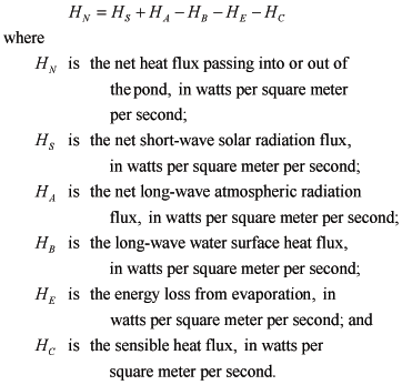
The net heat transfer across the air-water boundary is the summation of multiple heat flux terms and is given as:
 (1)
(1)
Heat transfer from rainfall to the ponds is small and is not included (Webb and Zhang, 1997). The heat transfer terms in equation 1 are calculated as hourly average heat fluxes. The only directly measured heat flux term in equation 1 is net short-wave solar radiation, HS,, which was measured by California Irrigation Management Information System (CIMIS) at the Fremont station (fig. 1). The available record of hourly values of HS are included in the HourlyData worksheet. The other terms in equation 1 are calculated as defined below:
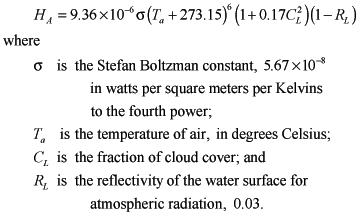
Long-wave atmospheric radiation, HA, varies with the moisture content of the air and is determined in the model using the following equation (U.S. Geological Survey, 1954):
 (2)
(2)
Air temperature data were measured at the CIMIS Fremont station and are listed in the HourlyData worksheet. Cloud cover data were unavailable for the study area and were estimated using a procedure described in the ‘Input Data’ section of this report. Estimated fraction of cloud cover data also are listed in the HourlyData worksheet.
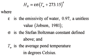
The long-wave water surface heat flux, HB, is the heat lost from the water surface, and it is calculated by the Stefan-Boltzman equation:
 (3)
(3)
Emissivity corrects for the fact that the water body is not an ideal blackbody radiator. The average pond temperature is calculated by the model during the previous hourly time step.
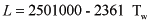
The energy loss from evaporation, HE, is calculated by the following equation (Jobson, 1981):
 (4)
(4)
where L is the latent heat of vaporization, in units of joules per kilogram, calculated as:
 (5)
(5)
and the hourly average evaporation rate, E, in meters per second, is calculated by the model (Lionberger and others, 2004).
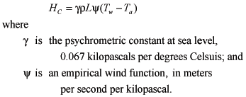
The sensible heat flux, HC, which is heat that is conducted and convected between the water surface and the air, is calculated from the following equation (Jobson, 1981):
 (6)
(6)
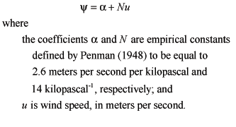
The wind function is determined from the following equation:
 (7)
(7)
Wind speed data were measured at the CIMIS Fremont station and are listed in the HourlyData worksheet.
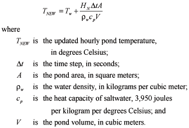
Once the net heat flux, HN, is determined, the hourly pond temperature is calculated as:
 (8)
(8)
Calculated hourly pond temperatures are averaged over 24 hours to obtain a daily average pond temperature. Daily minimum and maximum average pond temperatures are the lowest and highest simulated hourly pond temperatures during the 24-hour period. Minimum and maximum daily temperatures are important ecological factors for many aquatic organisms; therefore, these data are critical criteria for meeting habitat goals.
The temperature subroutine does not consider the effects of temperature difference between incoming water transfers and pond water. These effects are likely to be small because the volume of water transfers typically is small, compared to the volume of the pond (less than 1 percent for daily pond-to-pond water transfers), and any incoming water transfer is assumed to be dispersed instantly within the pond. Although the volume of incoming water from the slough can be significant (up to 30 percent of daily pond A9 volume), no long-term slough water temperature data currently are available. Point measurements taken by the USGS almost simultaneously in Alviso Slough and pond A9 indicated little temperature difference. On that basis, the effects of temperature difference between incoming slough water and pond water also are considered to be small.
The temperature subroutine was validated by comparing simulated temperatures to measured pond temperatures on hourly and monthly timescales. Two data sets were used to validate the temperature subroutine; temperature data collected every 12 seconds over a 1-month period to validate hourly temperature simulations and data collected monthly over a 27-month period to validate monthly temperature simulations. Sub-hourly temperature data from pond 3 of the Napa salt ponds in North San Francisco Bay (fig. 2) were used because continuous data were unavailable for the Alviso salt ponds. Monthly data from the Alviso salt ponds were used, but the CIMIS Fremont weather station was not active during the data-collection period. Consequently, historical meteorological data from 1993 to 1995 were used to simulate pond temperatures measured during 2003–2005.
Validation of the temperature model on the hourly time scale was performed using the temperature data collected continuously in pond 3 of the Napa–Sonoma Salt Pond Complex in May 2001 (J. Bricker, written commun., formerly of Stanford University 2004). Data were collected in pond 3 along a transect at three different depths at each of three locations (fig. 2) and averaged spatially (nine-point mean) and then averaged temporally over 60 minutes to obtain a single average pond temperature for each hour.
Hourly average pond temperatures were simulated by SPOOM using meteorological data from the CIMIS Carneros weather station (#109) and compared with the measured data (fig. 3). The simulated temperatures have similar diurnal temperature patterns as the measured data, although simulated values were less than measured values by an average of 1.0°C. Some of this apparent bias in simulation may result from the assumption that measured temperatures at different depths along a single transect represent an average pond temperature. The error bars shown in figure 3 are based on the standard deviation of the temperature measurements at the nine points along the transect and indicate an average variation of about 0.3°C. Additional once-monthly measurements of temperature at five discrete locations in Pond 3 from April 1999 to October 2001 showed an average standard deviation among the five in-pond locations of about 1.5°C. On this basis, the average difference between simulated and measured temperatures for the validation appears reasonable, and no model adjustments were made to try to achieve a better fit to measured data.
Validation of the SPOOM temperature model on the monthly time scale was performed using temperature data measured in pond A14 from May 2003 to August 2005 during the daytime at monthly intervals. Measurements were taken from a minimum of three discrete locations in the pond and averaged to obtain an average pond temperature (U.S. Fish and Wildlife Service, 2006).
SPOOM is not configured to simulate the pond temperatures from May 2003 to August 2005, because meteorological data for that period are unavailable from the CIMIS weather station at Fremont. Instead, the temperature model was validated using historical meteorological data for a period (May 1993 to August 1995) that was considered to be similar to the May 2003 to August 2005 temperature data-collection period. Simulated daily average and daily maximum temperatures are compared to the measured once-monthly average temperatures in figure 4. Simulated daily maximum temperature is considered to provide a better comparison to the measured values because temperature was measured only during the day and in shallow water near the shore where temperatures probably are higher than the pond average. Although the simulated temperatures do not perfectly match the measured temperatures, simulated data show month-to-month variability in average pond temperature that is very similar to variability shown by measurements. On this basis, using historical meteorological data from previous years to simulate future, hypothetical pond temperatures is considered to provide reasonable results. Simulated results were not adjusted to fit the measured data.
The previous version of SPOOM simulated daily volume and salinity of a single pond. SPOOM has been modified to simulate conditions in ponds A9–A17, simultaneously. The Alviso pond system is surrounded by tidal sloughs, so tidal elevations in the sloughs are used as boundary conditions for ponds with slough connections. Pond-to-slough discharge through culverts is controlled, in part, by the slough water-surface elevation. Flow rates through the culverts are calculated hourly to account for changing tidal and pond water-surface elevations and summed over 1 day. SPOOM calculates the hydraulic head and the resulting flow through the culverts using rating curves. Rating curves are included for culverts with weir boxes, culverts with flap gates, new culverts with screw gates, old culverts with screw gates (36 and 48 in.), and the siphon connecting ponds A15 and A16.
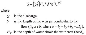
Discharge from ponds to the tidal sloughs is controlled by weir boxes and by culverts equipped with combination gates at each end. Combination gates can function as either a flap gate to allow unidirectional flow or as a screw gate to prevent flow or allow bidirectional flow. Figure 5 illustrates an example of unidirectional culvert flow. Weir boxes, located inside the pond and surrounding the culvert entrance, are roughly 9 ft x 9 ft x 6 ft and made of cast concrete with six bays of removable wooden weir boards (fig. 6). If the weir boards are fully removed, the culverts control pond discharge to the slough; otherwise, the weir box is the dominant hydraulic control. One possible exception is during high tide when the weir is submerged. The effect of the culvert would again dominate. To account for this the model calculates flow as culvert discharge and also as weir discharge and assumes the smaller of the two as the discharge for that hourly period.
Weir discharge can be determined from a standard weir equation (Sturm, 2001) as
 (9)
(9)
and
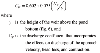 (10)
(10)
Culvert discharge from pond to slough without the use of a weir box is affected by tidal conditions in the slough. A series of culvert discharge measurements in pond A3W (fig. 1) during a tidal cycle was used with a form of the Bernoulli equation to develop a relation between culvert discharge from a pond to a slough and the difference in water-surface elevations of the pond and slough. The discharge relation is assumed valid for the other discharge ponds in the Alviso Salt Pond Complex because their discharge structures are similar to that of pond A3W. Culvert discharge was measured using a downward-looking acoustic Doppler current profiler (ADCP). The ADCP was mounted in a small aluminum sled and towed across the pond about 3–15 ft upstream from, and perpendicular to, the culvert inlet. Measured point velocities were integrated over depth and path length to compute total culvert discharge. Culvert discharge also can be calculated using the following form of the Bernoulli equation applied to the upstream and downstream ends of the culvert (Shellenbarger and others 2007):
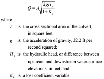 (11)
(11)
This equation assumes the culvert is flowing full as a result of the backwater conditions produced by a hinged flap gate on the slough side of the culvert. The measured pond discharges and values of hydraulic head (Hp) were used in equation 9 to solve for the loss coefficient, KL, representing all energy losses, including entrance, friction, contraction, and exit as well as unquantifiable losses associated with the flap gates. The loss coefficient does not include losses associated with the screw gate. The model assumes that the screw gate is only used to completely close the culvert to prevent flow (only for culverts connecting ponds to sloughs), otherwise the screw gate is kept fully open, as shown in figure 5. The loss coefficient was found to vary with hydraulic head in a manner best described by two best-fit equations, (fig. 7). At low heads (Hp < 0.626 ft), KL exponentially decreases with increasing head,
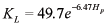 (12)
(12)
This probably is due to the flap gate opening further as head increases. At high heads (Hp > 0.626 ft), KL linearly increases with an increase in head.
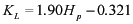 (13)
(13)
The exponential function defined by equation 10 and the line defined by equation 11 intersect at Hp = 0.626 ft.
When slough water-surface elevations fall below the elevation of the inside bottom of the culvert, or culvert invert, the flap gate is the dominant hydraulic control. Therefore, tidal slough water-surface elevations that fall below the elevation of the culvert invert are neglected and the hydraulic head is measured as the difference between the pond water-surface elevation and the culvert invert elevation. Culvert invert elevations are given in table 3.
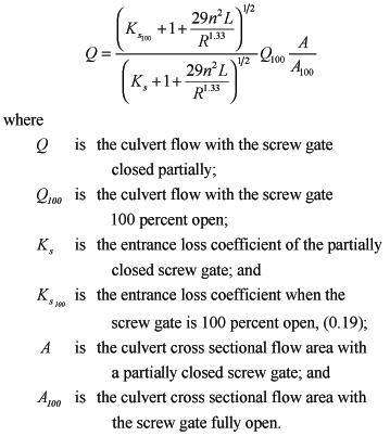
Pond-to-pond discharge is controlled by a series of culverts equipped with screw gates to regulate flow. Some of these culverts were in place before the ISP period, and some new culverts were installed for managing the ponds during the ISP period. Because older culverts can be filled partially with debris, they will not flow to their full capacity as would new culverts. Consequently, pond-to-pond culvert discharge is simulated in two ways: using theoretical flow-rating curves for new culverts and measured flow-rating curves for existing culverts.
Theoretical flow rating curves used for new culverts are based on the assumption that the culvert is submerged fully and flowing under outlet-control conditions (American Society of Civil Engineers, 1992). The rating curve is a function of the hydraulic head across the culvert and is of the form
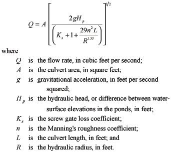 (14)
(14)
Manning’s roughness coefficient values are available from a number of sources and often are presented as a range. The value used in this study (0.022) is at the mid-point of a range for corrugated metal pipe given by White (1999; table 10.1).
The screw gate loss coefficient, Ks, varies, depending on the size of the culvert-flow area. The ScrewGates worksheet allows the user to specify a percent of the culvert cross-sectional area, P, open to flow for a specific day for pond-to-pond connections. Based on gate valve loss coefficients listed by Jeppson (1976; table 3-1), Ks can be calculated from P using the following equation (fig. 8):
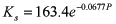 (15)
(15)
At fully open, Ks is 0.19 and then increases exponentially with decreasing flow area.
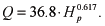
Rating curves for old culverts with screw gates were developed from culvert discharge measurements using an ADCP and measured hydraulic heads (Hp, difference between upstream and downstream pond elevations). Measurement data were grouped by culvert dimensions, and discharge was related to hydraulic head using a best-fit exponential equation. The resultant rating curve for the 36-in. culverts was (fig. 9):
 (16)
(16)
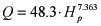
and the rating curve for the 48-inch culverts is (fig. 10):
 (17)
(17)
An exponential rating curve also was determined (not shown) for the siphon-connecting ponds A15 and A16:
 (18)
(18)
Only three measured flow rates were used to determine equation 16.
Culvert discharge was measured only when the screw gates were open fully. To calculate culvert discharge through a partially open screw gate on an old culvert, the ratio of discharge with a partially open gate to discharge with a fully open gate was assumed to be the same as that for a new culvert. On that basis, dividing equation 12 for a partially open screw gate condition by equation 12 for a fully open screw gate condition and rearranging terms provides the following equation for calculating culvert discharge with a partially open screw gate:
 (19)
(19)
The Geometry worksheet lists area and volume for ponds A9–A17 as functions of water-surface elevation, relative to vertical datum NAVD 88. The areas and volumes were calculated using ArcGIS geographic information system software (ESRI, Redlands California). Initially, boundaries for ponds A9–A17 were delineated by on-screen digitization using high-resolution digital orthophotos (0.3-meter pixel resolution) at a scale of 1:1,000 as a base layer. The orthophotos were obtained online from the USGS Seamless Data Distribution Delivery website (http://gisdata.usgs.net/website/seamless/viewer.php), and the pond boundary polygons were digitized for the wetted perimeter, as observed in the orthoimagery, of each pond.
Bathymetric data for the Alviso ponds were obtained from the USGS Western Ecological Research Center as a series of spreadsheet files containing positional data as latitude, longitude, and elevation for points within each pond (Takekawa and others, 2005). These data were referenced to the horizontal and vertical datums, NAD 83 and NAVD 88, respectively. The spreadsheet data for each pond then were converted into point shapefiles using ArcGIS.
LiDaR (Light Detection and Ranging) elevation data, for an area including ponds A9–A17, were obtained from the Environmental Services Department of the City of San Jose (written commun., 2002). These data also were obtained in spreadsheet format and converted to point shapefiles. The horizontal and vertical datums were NAD 83 and NAVD 88, respectively. Data points located within the boundaries of the ponds then were eliminated from the dataset as they represented water-surface elevations rather than pond bottom elevations. The point shapefiles for the bathymetric and LiDaR data then were merged into a single point shapefile in ArcGIS. This file was converted to a Triangular Irregular Network (TIN) three-dimensional (3D) surface using the ArcGIS 3D Analyst extension and converted to a raster image. The raster image was clipped using each of the pond boundary polygons. The resulting raster images for each pond were analyzed using the 3D Analyst extension. Pond surface area and volume were determined by using a horizontal plane to represent the pond water surface. Calculations were performed by raising the water-surface elevation in 0.1-foot increments, based on the minimum and maximum elevation values for each pond TIN. The results of these calculations were exported automatically from the GIS software as text files which, subsequently, were converted into spreadsheet files.
SPOOM enables the user to perform simulations referenced to the NAVD 88 or NGVD 29 vertical datums by using a pull-down list located on the Main worksheet. A conversion factor (-2.69 ft or 0.82 m) for converting NGVD 29 elevations from NAVD 88 elevations was determined using VERTCON (http://www.ngs.noaa.gov/TOOLS/Vertcon/vertcon.html, accessed on August 30, 2007) and is applied in the model code. Thus, simulations can be made using either vertical datum without the need to change any geometry data.
The worksheet HourlyData includes hourly average values of solar radiation, air temperature, fraction of cloud cover, wind speed, and evaporation for water years 1992–96, 1998 and 1999. Water year 1997 is excluded because of missing data. These data are necessary for the temperature subroutine. The meteorological data are historical data from the CIMIS weather station at Fremont (#100), except for the fraction of cloud-cover data and freshwater evaporation data.
Cloud-cover data were unavailable for the study area. A method was developed to estimate this parameter using solar radiation data measured by CIMIS. A 30-day centered mean and standard deviation of the mean of daily average solar radiation were calculated. The range of values used to calculate the mean and standard deviation of the first and last 14 days of the record were truncated so that an equal number of days were considered before and after the day being calculated. Fraction of cloud cover for each day was considered to be zero if solar radiation for the day was less than the average value minus one standard deviation, 1.0 if the solar radiation was greater than the average value plus one standard deviation, and ![]() for all values of solar radiation in between.
for all values of solar radiation in between.
The value of ![]() was chosen based on the assumption that the mid-range of fraction of cloud cover should correspond to the long-wave atmospheric radiation halfway between that for no cloud cover and that for complete cloud cover. The heat equation (eq. 2) indicates that long-wave atmospheric radiation is proportional to the square of the fraction of cloud cover. On that basis, the square of the fraction of cloud cover, midway between 0 (no cloud cover) and 1.0 (complete cloud cover), is 0.5, and the square root of 0.5 is
was chosen based on the assumption that the mid-range of fraction of cloud cover should correspond to the long-wave atmospheric radiation halfway between that for no cloud cover and that for complete cloud cover. The heat equation (eq. 2) indicates that long-wave atmospheric radiation is proportional to the square of the fraction of cloud cover. On that basis, the square of the fraction of cloud cover, midway between 0 (no cloud cover) and 1.0 (complete cloud cover), is 0.5, and the square root of 0.5 is ![]() . At most, the fraction cloud cover coefficient affects the long-wave atmospheric radiation term by 17 percent (eq. 2). Therefore, the model results are relatively insensitive to the coefficient estimates employed here.
. At most, the fraction cloud cover coefficient affects the long-wave atmospheric radiation term by 17 percent (eq. 2). Therefore, the model results are relatively insensitive to the coefficient estimates employed here.
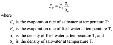
Hourly freshwater evaporation rates were calculated using the Combined Aerodynamic and Energy Balance Method (Chow and others, 1998; Lionberger and others, 2004) and meteorological data from the CIMIS weather station at Fremont (#100). Salinity increases water density, thereby reducing the value of evaporation to less than the freshwater value. To account for the effect of salinity on evaporation, a correction factor is applied in the model to reduce evaporation.
 (20)
(20)
The Rainfall worksheet contains daily rainfall rates from the closest rainfall gage to the ponds, Guadalupe Slough RF 16, operated and maintained by the Santa Clara Valley Water District (SCVWD) (figs. 1 and 11). The driest year of the record is water year 1994, with 71 percent of normal precipitation and the wettest year of record is water year 1998, with 163 percent of normal. Normal is defined in this report as the mean of the annual rainfall values for the 1992–1996 and 1998–1999 period of record included in the model. The model user also can enter custom rainfall data by choosing ‘Custom’ from the rainfall pull-down box on the Main worksheet and by entering a data series, in units of millimeters per day, in column C of the Rainfall worksheet. The range of dates specified by the user in the start date and end date pull-down boxes in the Main worksheet must be consistent with the dates of custom rainfall data.
Although the use of custom rainfall enables the user to simulate pond conditions for rainfall data outside the period of record in the model, other meteorological data used in the model are for the available period of record at the CIMIS station at Fremont only and, thus, may not be consistent with the custom rainfall.
Hourly slough water-surface elevation is the boundary condition for ponds with culverts connecting to the sloughs. Long-term water-surface elevation data were not available at any of the Alviso pond culverts connecting to the sloughs. Instead, tidal elevation data measured every 12 minutes from January 31 to April 29, 2004, by Moffatt and Nichol Engineers (2005) in Coyote Creek at Power Tower (fig. 1) were used to predict water-surface elevations for the dates when meteorological data were available (water years 1992–96, 1998, and 1999). Tidal harmonic analysis was applied to the data using T_TIDE for MATLAB (Pawlowicz and others, 2002). Using the tidal harmonic constants extracted from this dataset, predictions of hourly tidal water-surface elevations were made for the period of record included in the model using T_PREDIC for MATLAB (Pawlowicz and others, 2002). Data from the Power Tower site (fig. 1) were used in this analysis because its location is the closest tidal elevation monitoring site to the ponds, located no more than 7 km from any of the slough-to-pond culverts. The model is based on the assumption that the tidal elevation at Power Tower represents tidal elevations in the sloughs at all culverts in the Alviso system. Tidal range decreases upstream of the Bay, however, and tidal data at Power Tower may not represent the tidal elevation at ponds A16 and A17 as well as at A9 and A14. Errors associated with the assumption that tidal elevations are the same throughout the sloughs are unknown. Hourly predicted tidal elevations are listed in the HourlyData worksheet.
In summer and fall, slough salinities vary diurnally with the tides, with higher salinities at high tide and lower salinities at low tide owing to freshwater effluent from the San Jose/Santa Clara Water Pollution Control Plant. In winter and spring, slough salinities are more variable, depending on storm-water runoff. Since flows into the ponds are restricted during the winter and spring, SPOOM accounts only for slough salinities in the summer and fall. Continuous salinity data were measured half-hourly by the City of San Jose ESD at the Coyote Creek railroad trestle (SB04) from October 16, 1997, to October 30, 1997 (fig. 1, City of San Jose, written commun., 1997). This location was chosen because it is the closest downstream measurement site to the ponds and is centrally located between ponds with slough-connecting culverts. Salinities measured on the hour were plotted against hourly slough water-surface elevation estimated using T_PREDIC for MATLAB (Pawlowicz and others, 2002) to formulate a rating curve to estimate slough salinities for use in the model (fig. 12). Because the salinity record is so short, the accuracy of the salinity prediction during other times of the year is unknown. The data show hysteresis between flood and ebb tides. As a result, two rating curves were developed for application to flood tide
 (21)
(21)
and to ebb tide
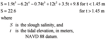 (22)
(22)
in column H of the HourlyData worksheet, estimates of hourly tidal direction of flood or ebb are listed, on the basis of whether the water level is increasing or decreasing. The model accesses the hourly tidal direction and tidal elevation given in column G, and applies the appropriate rating curve.
The only pond able to receive inflow from the sloughs in winter is pond A16. The culvert connecting pond A16 to the slough is located near the wastewater treatment plant outlet to the slough. Continuous salinity measurements taken in summer just upstream from the A16 culvert indicate that the salinity is zero most of the time. Slough salinity will be even fresher in winter owing to storm runoff. Therefore, the salinity of slough inflows into pond A16 during winter is assumed to be zero.

![]() U.S. Department of the Interior | U.S. Geological Survey
U.S. Department of the Interior | U.S. Geological Survey
URL: https://pubs.usgs.gov/sir/2007/5173
Page Contact Information: Publications Team
Page Last Modified: Thursday, 01-Dec-2016 19:57:51 EST
