Scientific Investigations Report 2008–5076
U.S. GEOLOGICAL SURVEY
Scientific Investigations Report 2008–5076
The governing equations for three-dimensional, baroclinic circulation and the transport of scalar variables in a lake include the conservation equations of mass and momentum, a kinematic free-surface equation (derived from mass conservation), an equation of state relating density to temperature, and a conservation equation for each scalar variable. The lake is assumed to be sufficiently large for a Coriolis acceleration term to be included in the momentum equations. To simplify the governing equations, the water is assumed to be incompressible and it is assumed that the Boussinesq approximation applies. In Cartesian coordinates, the mass conservation equation is
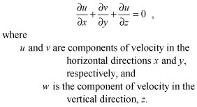 (1)
(1)
After integrating over depth and applying the kinematic condition at the free surface, the mass conservation equation becomes
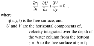 (2)
(2)
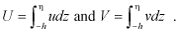 (3)
(3)
The momentum conservation equations in three spatial dimensions are
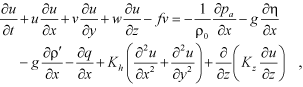 (4)
(4)
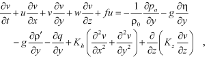 (5)
(5)
and
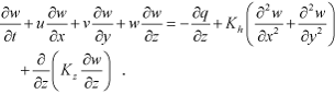 (6)
(6)
The Coriolis parameter f is assumed constant over the domain. Kz and Kh and are the vertical and horizontal viscosity coefficients, respectively, ρ0 is a constant reference density of water (1,000 kg/m3), g is gravitational acceleration (9.81 m s-2), and ρ' is the vertically integrated and normalized deviation from reference density. The above equations have been derived by decomposing the pressure P into a hydrostatic component, dependent on the free-surface elevation η and the spatially varying density ρ, and a nonhydrostatic component q as:
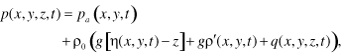 (7)
(7)
where
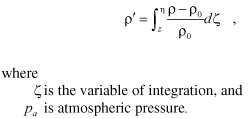 (8)
(8)
The equation for conservative transport of a scalar variable (including heat and solute) with concentration C is:
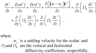 (9)
(9)
The final equation is the equation of state, which in the general case relates density to temperature and salinity. In this freshwater application the equation of state is an empirical relation that relates density in kg m-3 only to water temperature Tw in °C (Gill, 1982):
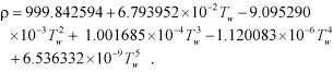 (10)
(10)
Equations (2) through (10) are the governing equations solved within the computational core of the UnTRIM model. If the water density can be approximated as constant (barotropic flows), the scalar transport equation (9) is uncoupled from the momentum equations (4), (5), and (6). When the hydrostatic approximation is made, the horizontal gradients of q drop out of equations (4) and (5), and equation (6) is replaced by the hydrostatic approximation.
The governing system of equations can be solved efficiently by a semi-implicit finite-difference method that is computationally fast, accurate, and stable over a regular computational mesh as discussed by Casulli and Cheng (1992) and Casulli and Cattani (1994). A weak Courant-Friedrich-Lewy (CFL) stability condition is imposed on the computational time step due to the explicit treatment of the horizontal diffusion in the momentum equations. If density stratification in the lake is considered, the transport equations are coupled with the momentum equations through the density gradient terms. In this case, the density gradients in the momentum equations and the mass conservation of the scalar variables (including heat and solute) are solved explicitly. The resulting numerical scheme is subject to an additional weak CFL stability condition on the computational time step due to the explicit treatment of the transport equation and the baroclinic pressure terms in the momentum equations.
The governing equations are solved in physical space without invoking any coordinate transformation in the horizontal or vertical directions. The stability properties of the governing partial differential equations are controlled by using a semi-implicit finite-difference scheme (Casulli, 1990; Casulli and Cheng, 1992); the resulting numerical algorithm is robust and computationally efficient. Traditional finite-difference schemes resort to refining the rectangular finite-difference mesh when a complicated domain is encountered in order to resolve the flow distributions in narrow and confined regions. The resulting fine-resolution grids in broad and open regions are unnecessary, and the computational mesh consumes a large portion of computing resources, which is not computationally efficient. In the UnTRIM model, the semi-implicit finite-difference method is applied over an unstructured grid (Casulli and Zanolli, 1998; Casulli and Walters 2000) in which fine grid resolutions are used in complex regions, and relatively coarse grids are used in broad and open areas.
When a computational mesh is created, the horizontal domain is covered by a set of nonoverlapping convex polygons. Each side of a polygon is either a boundary line or a side of an adjacent polygon. The center of each polygon is defined such that the segment joining the centers of two adjacent polygons intersects the side shared by the two polygons and is orthogonal to it (fig. 2). The center of a polygon does not necessarily coincide with its geometrical center, except in special cases such as rectangular finite-difference grids and grids of uniform equilateral triangles. This type of computational mesh is called an unstructured orthogonal grid (Casulli and Zanolli, 1998; Casulli and Walters, 2000). In an unstructured grid representation within the UnTRIM model, each polygon has either three or four sides. Each polygon, side, and vertex in the grid is assigned a unique number. The x–y coordinates of the vertices of each polygon must be specified, as well as the information that relates each polygon to its vertices and sides.
In the vertical direction, the water body to be modeled is divided into layers by horizontal planes. The polygons between the horizontal planes become a stack of prisms whose thickness is the prescribed layer thickness. The water-surface elevation is assumed to be uniform within each polygon and is defined at the center of the polygon. The velocity component normal to each face of a prism is assumed to be uniform over the face. The velocity is defined at each vertex in the middle of each layer, and the spatial distribution of velocity through the prism is obtained by interpolating between the velocities at the vertices. Finally, the water depth below each polygon is specified and assumed uniform on each side.
The unstructured orthogonal grid for UKL (fig. 3) was created and optimized with the JANET software (Lippert and Sellerhoff, 2006). This software enables semiautomated creation of an initial grid, followed by manual fine-tuning of individual polygons that are identified by tests within the software to be outside of a prescribed tolerance for orthogonality. The resulting grid for UKL has 8,389 polygons, 4,555 vertices, and 28 layers of 0.5 m thickness. Because most of the lake is shallow, however, the number of active prisms in each layer varies from more than 8,000 in each of the top 3 layers to less than 100 in each of the 11 deepest layers of the grid. The length of the sides of the polygons varies from approximately 100 m in areas along the trench where the bathymetry changes rapidly to approximately 400 m in the open areas of the lake.
A semi-implicit finite-difference scheme is used to obtain an efficient numerical algorithm for which stability is independent of free-surface gravity waves, wind stress, vertical viscosity and bottom friction, for both the hydrostatic (Casulli and Walters, 2000; Casulli, 1990) and nonhydrostatic case (Casulli and Zanolli, 2002; Casulli, 1999a, Casulli, 1999b). The momentum equations (4)–(6) are finite-differenced in the direction normal to each vertical face of each computational prism (along oa, ob, and oc in fig. 2). The momentum equations relate the gradient of water-surface elevation between adjoining prisms to the face velocity on the common face between these prisms. The vertical mixing and the bottom friction are discretized implicitly in time for numerical stability, whereas an explicit finite-difference operator is used to solve the wind stress and the advection and horizontal dispersion terms. This operator can take several particular forms; an Eulerian–Lagrangian scheme is used in UnTRIM (Casulli and Cheng, 1992). For stability, the implicitness factor θ must be in the range 1/2 ≤ θ ≤1 (Casulli and Cattani, 1994). In the vertical direction, a simple finite-difference discretization that does not require uniform layers is adopted. The vertical thickness of the top and bottom layers can vary spatially and the thickness of the top layer also can vary with time. The vertical thickness of the top layer is allowed to become zero, in order to accommodate the drying of cells.
The free-surface equation (2) is discretized semi-implicitly (Casulli and Cattani, 1994; Casulli and Walters, 2000), and only the face velocities are needed to complete the finite volume balance of total volume below each polygon. The surface elevation at the center of each polygon is determined by substituting the finite-differenced momentum equations on all faces of the polygon into the continuity equation. The resulting matrix equation governs the water-surface elevation over the entire domain. This matrix equation is strongly diagonally dominant, symmetric, and positive definite; thus its unique solution can be efficiently determined by preconditioned conjugate gradient iterations until the residual norm becomes smaller than a given tolerance (Golub and van Loan, 1996). Once the free surface of the entire domain for the next time level has been calculated, the normal velocities on the faces of the prisms are calculated by back substitution. The details of the finite-difference equations are not reproduced here and readers are referred to Casulli and Walters (2000).
The transport equation (9) for scalar variables is solved explicitly by using the velocity field obtained from the previous time step. An explicit finite-volume discretization that both conserves mass and guarantees that the solution will be bounded by the maximum and minimum of the initial and boundary values is used. In addition, a “flux limiter” is used in the discretization of the equation in order to limit numerical diffusion and preserve high accuracy at grid resolutions that are well-matched to the domain (Casulli and Zanolli, 2005). The flux limiter used in the simulations discussed here is the Superbee function (Roe, 1986).
In summary, the numerical solution scheme used in the computational core of UnTRIM to solve the governing equations is designed to achieve computational efficiency while retaining the accuracy of the solution. For the UKL simulations discussed in this report, the hydrostatic approximation was made. The simulations included the transport of three scalar quantities: turbulent kinetic energy, the rate of dissipation of turbulent kinetic energy, and heat. The equations describing the transport of each of these scalars are discussed below. Using the numerical solution scheme described above, the UnTRIM model required an average of 1.3 seconds of computational time per 2-minute simulation time step to solve the governing equations on the UKL grid, using a Dell 620 Latitude 1.66 GHz notebook computer with an Intel T2300 dual processor. A list of symbols used in this report is provided in table 1.
The vertical turbulent dispersion of momentum and diffusion of heat are calculated within the model as spatial and temporal functions of two localized flow characteristics—turbulent kinetic energy k and the rate of dissipation of turbulent kinetic energy ε. Equations for the transport of these two turbulence characteristics can be written as:
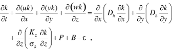 (11)
(11)
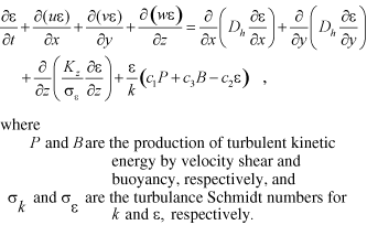 (12)
(12)
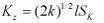
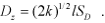
The implementation of this two-equation turbulence closure model within UnTRIM is accomplished by using the generic length-scale approach of Umlauf and Burchard (2003) and Warner and others (2005), which provides a convenient and flexible means for implementing a wide variety of two-equation turbulence closure models. The choice of the generic coefficients—c1, c2, and c3—that apply to the source and dissipation terms for the length-scale parameter ε determines which turbulence closure model is implemented. The k – ε model (Rodi, 1993) was used in the simulations presented in this report. In accordance with Warner and others (2005), the choice of c1 = 1.44, c2 = 1.92, and c3 = –0.52 was used to implement the k – ε model in the case of stable stratification (B < 0). In the case of unstable stratification (B > 0), the weak thermal stratification in UKL generally resulted in too much mixing when buoyancy was considered to be a source of k and ε, so the buoyancy term B was set to zero in equations (11) and (12) when unstable stratification occurred. Equations (11) and (12) are solved within the model and the turbulent diffusivities, Kz and Dz for momentum and constituent transport, respectively, are calculated at each time step as:
 (13)
(13)
and
 (14)
(14)
The length scale of the turbulent eddies, l, is related to ε by
![]() , where
, where ![]() is a constant that depends on
is a constant that depends on
the stability functions used. The stability functions SK and SD are algebraic functions of k and ε that are derived by converting the system of differential equations for the second-order moments of turbulent quantities to a system of algebraic equations, thus eliminating a great deal of computational effort. The stability functions used in this application were those derived by Kantha and Clayson (1994). The solution of the equations (11) and (12) for k and ε is accomplished sequentially at each time step. The advective and diffusive transport is solved as described above for a scalar quantity. Then P, B, and ε are calculated from the velocity and density gradients, and then the source and sink terms of equations (11) and (12) are used to update k and ε. The implementation of this turbulence closure in UnTRIM is described by Celebioglu and Piasecki (2006a and 2006b).
The shear stress at the surface of the water column, ![]() , is specified in terms of a surface drag coefficient C10:
, is specified in terms of a surface drag coefficient C10:
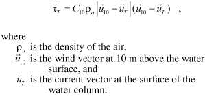 (15)
(15)
The surface drag coefficient is in general an increasing function of the wind speed, and various formulations have been proposed and evaluated (Garratt, 1977; Smith and Banke, 1975). At very low wind speeds (less than about 3 m s-1) experimental evidence shows that the wind surface drag coefficient increases with decreasing wind speed (Wuest and Lorke, 2003). In this application, an increasing C10 at low wind speeds did not bring the simulated currents closer to observed currents, and the following function for C10 was used: ![]() for 10-m wind speeds less than 15 m s-1
for 10-m wind speeds less than 15 m s-1
and ![]() for greater wind speeds. The value of a was treated as a calibration parameter, although the final choice of a = 0.0005 was the value proposed by Wu (1969).
for greater wind speeds. The value of a was treated as a calibration parameter, although the final choice of a = 0.0005 was the value proposed by Wu (1969).
The shear stress at the sediment/water interface ![]() is defined in terms of a bottom friction coefficient rB and the near-bottom current speed
is defined in terms of a bottom friction coefficient rB and the near-bottom current speed ![]() as:
as:
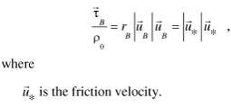 (16)
(16)
Within the bottom logarithmic profile layer, the speed of the currents at distance z' away from the interface is given by (Schlichting, 1955):
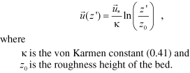 (17)
(17)
Combining these two expressions allows the solution of rB in terms of the distance zB of the lowest computational grid point away from the bottom, where is defined:
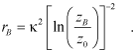 (18)
(18)
The effort to develop an UnTRIM model of UKL began in 2003, and these efforts were reasonably successful at reproducing the hydrodynamics of the lake (Cheng and others, 2005). The early simulations showed that the currents in the lake were highly responsive to wind forcing at the surface, and it was determined that the biggest improvement in model performance would be obtained by generating a spatially accurate surface wind, rather than using a uniform surface wind over the entire lake. By 2005, additional monitoring sites had been established around the lake, as described below. Observations from these monitoring sites showed that the surrounding land topography influences the wind field over the lake, as evidenced, for example, by the fact that the prevailing wind direction over the northern part of the lake is westerly, but is northwesterly over the southern part of the lake (Hoilman and others, 2008).
An objective analysis model of the atmospheric boundary layer was used to interpolate the observations from the various wind-monitoring locations to a uniform grid (500-m spacing, both east-west and north-south) over the lake (Ludwig and others, 1991). The procedure for doing this involves starting with an initial “guess” interpolation and then modifying the initial guess iteratively to satisfy mass continuity. When temperature profiles in the lower atmosphere are available, the thickness of the surface flow is adjusted to the height at which the kinetic energy in the wind is equal to the work done against buoyant restoring forces. Surface winds flow over features of the terrain that are lower than this thickness, and around features that are higher than this thickness. Because temperature soundings in the near-surface around UKL are not part of the routine data collection around the lake, the full functionality of this model was not used. Instead, a stable and invariant adiabatic temperature profile in the atmospheric boundary layer was assumed.
Source/sink terms that describe the transfer of heat across the air/water interface were added to the equation for conservative transport of a scalar variable (eq. 9). Surface terms include incoming shortwave and longwave radiation, outgoing longwave radiation, evaporative cooling, and conduction/convection. Computationally, all of these terms except for incoming shortwave radiation are included in the surface boundary condition. Incoming shortwave radiation is treated as an internal source/sink term that allows the radiation to be absorbed through a finite distance in the upper layers of the model water column rather than only at the air/water interface. The three-dimensional equation describing the transport of heat is:
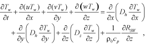 (19)
(19)
where Tw is the water temperature, and
 (20)
(20)
is the rate of temperature change at any depth z due to local absorption of shortwave radiation. The shortwave radiation at any depth z in the water column is given by:
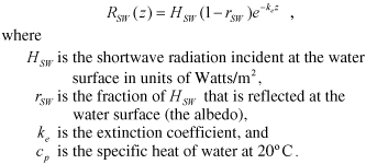 (21)
(21)
The internal source/sink term is applied to the water temperature outside of the computational core of the model, with the result that at each time step, temperature over the entire domain is first updated to an intermediate value by physical transport; then, the change in heat resulting from the absorption of shortwave radiation is applied to the intermediate temperature.
The rest of the surface heat transfer terms are treated computationally as a boundary condition because they apply directly at the water surface. The boundary condition at the water surface is:
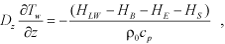 (22)
(22)
where HLW , HB, HE , and HS are the incoming longwave radiation, reflected longwave radiation, evaporative heat flux, and sensible heat flux, respectively, all with units of Watts/m2. This boundary condition is updated at every time step and the new value is supplied to the computational core of UnTRIM.
Of the surface heat transfer terms, only the incoming shortwave radiation HSW is directly measured. The rest of the surface terms are calculated within the model at each time step by using standard formulations (McCutcheon, 1989; Martin and McCutcheon, 1999). Atmospheric long wave radiation is calculated from the Stefan-Boltzmann law, modified for the emissivity of the air:
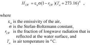 (23)
(23)
The emissivity of the air is calculated as:
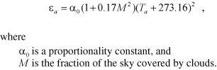 (24)
(24)
Back radiation from the water surface also is calculated from the Stefan-Boltzmann law:
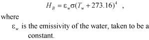 (25)
(25)
Evaporative heat loss is calculated as:
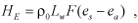 (26)
(26)
where
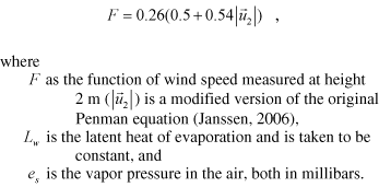 (27)
(27)
The saturation vapor pressure at the water-surface temperature is given by (Dingman, 2002):
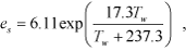 (28)
(28)
and the vapor pressure in the air is calculated from relative humidity rh as:
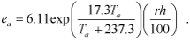 (29)
(29)
Sensible heat loss is often calculated from evaporative heat loss using the Bowen ratio:
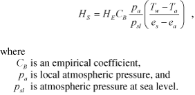 (30)
(30)
The sensible heat loss term is small compared to the other terms in eq. (22). In the UKL model the inclusion of this term tended to reduce the accuracy of the simulation, particularly during periods of atmospheric cooling when HS was negative, so sensible heat loss was not included in the model simulations presented in this report.

![]() U.S. Department of the Interior | U.S. Geological Survey
U.S. Department of the Interior | U.S. Geological Survey
URL: http://pubs.usgs.gov/sir/2008/5076
Page Contact Information: Publications Team
Page Last Modified: Thursday, 10-Jan-2013 18:48:16 EST
