Study Design and Methods

Surface- and ground-water quality was evaluated at several sites in each unit in 2003–05. Adjacent streams, Wood River and Sevenmile Canal (table 1, fig. 2), also were sampled for comparison. Sampling was concentrated during the growing season (approximately monthly May/June through September) with a few winter and early spring samples collected to characterize the non-growing season. Samples of flood-irrigation water were collected over a 3-day period in September 2003, when water from the adjacent property to the north was let on to the wetland. In 2005, samples were collected monthly from June to September.

A hydrologic budget for the Wood River Wetland was developed by collecting information on inflows, outflows, and changes in water storage for the wetland. Water-budget components were determined through measurement or estimation. Results of the water-budget analysis were used to calculate standing surface-water volume on each sampling date to quantify changes in water quality over time.

Field Methods

Water samples—Water samples were collected from adjacent streams at the Dike Road bridges (for Sevenmile Canal and Wood River) or at the Sevenmile Canal water control structure at the inlet to the wetland (fig. 2). Surface-water sites in the wetland were accessed by canoe or by wading. Discrete water samples were collected about 10–20 cm below the water surface. Although wind occasionally mixes the surface water, temperature stratification was sometimes observed, especially in the South Unit. Therefore, the discrete water samples may not fully represent the water quality throughout the water column.

Accessing canals for sampling at the Wood River Wetland (looking southeast). Photograph taken by John Duff, U.S. Geological Survey, August 2004.

In the North Unit, sampling started at the northwest corner and progressed toward the southeast corner pump station. In the South Unit, sampling order varied depending on water level, wind, and other conditions. Surface water was collected using a battery-operated peristaltic pump (Geopump^®) with Masterflex^® tubing. Occasionally, water samples were collected in 2-L amber polyethylene bottles and processed off site.

Water samples also were collected from eight ground-water piezometers (fig. 2) using a peristaltic pump and weighted Masterflex^® tubing. Wells were purged for at least 10 minutes (or until dry) by pumping approximately three water volumes from each well. Water samples were collected 12–24 hours after purging to allow fresh water to recharge wells. Prior to initial purging, water levels were measured with a calibrated electronic E-tape.

Water samples were analyzed for filtered and unfiltered (total) nutrients on 15 occasions. Dissolved organic carbon (DOC), select metals, and chloride (Cl) were analyzed less frequently. Bulk samples were shaken and subsampled into 125-mL bottles for total phosphorus (TP) and total Kjeldahl nitrogen (TKN). Samples for dissolved constituents, including ammonium (NH₄), nitrite plus nitrate (NO₂+NO₃), hereafter referred to as nitrate (NO₃), and dissolved Kjeldahl nitrogen (DKN) were filtered into 60-mL sample bottles (for NH₄, NO₃, and SRP), or a 125-mL bottle (for DKN). Filtered samples were processed through 0.45-µm filtration capsules attached directly to the peristaltic tubing or collected into a 60-mL syringe and filtered through 0.45-µm Acrodisk^® filters. DOC samples were filtered through combusted 0.7 µm GF/F filters (Whatman^®). Total nutrient samples (TKN and TP) were acidified with 1 mL sulfuric acid (H₂SO₄), and NH₄ and SRP samples were preserved with 100 µL concentrated hydrochloric acid (HCl) per 60-mL sample. Samples were packed on ice and shipped to the laboratories for analyses.

Field parameters—In-situ water temperature, specific conductance (SC), dissolved oxygen (DO), and pH were measured at most sites using a calibrated Hydrolab H20 or YSI 6600 multi-parameter probe, or an equivalent single-parameter meter. Readings occasionally were taken below the water surface and just off the bottom, but most readings were taken about 10–20 cm below the water surface. Vertical profiles of light intensity occasionally were collected to determine the light or photosynthetically active radiation (PAR) available for photosynthesis in the water column and to calculate the light extinction depth (where PAR is zero).

Ground-water piezometers—Eight piezometers (wells used to measure ground-water pressure head or to sample water quality at a point or specific depth range in the subsurface) were installed at four sites in July 2003 (fig. 2, table 2), according to the Oregon Water Resources Department guidelines for monitoring wells (Oregon Water Resources Department, 2001). Two nests consisting of three wells each (shallow, intermediate, and deep) were installed in the North and South Units, and two individual wells were drilled along the East and South Dike Roads (fig. 2). Slug tests were performed according to USGS protocols (Halford and Kuniansky, 2002) in the two dike road piezometers, PZ-WRDK, on the dike adjacent to Wood River, and PZ-AGDK, on the dike adjacent to Agency Lake. The slug tests were conducted to determine the hydraulic properties of the wetland soils and dike materials, and to estimate the rate of water flow through the dike materials and ground-water seepage through the wetland soils.

Construction of ground-water piezometers in the North Unit of the Wood River Wetland (looking north). Photograph taken by Charley Palmer, U.S. Geological Survey, August 2003.

Ground-water piezometer nest in the South Unit of the Wood River Wetland (looking west southwest). Photograph taken by Kurt Carpenter, U.S. Geological Survey, June 2004.

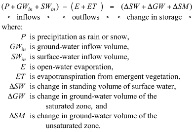
Material collected during well drilling included a wide range of coarse sediments (pumice pebbles and sand), silty loams, clays, peat, and a small amount of volcanic ash. The North Unit piezometers (PZ-NU1, PZ-NU2, and PZ-NU3) were installed in the northern corner of the wetland near an old corral. The shallow well (PZ-NU1) in this nest was completed in a pumice horizon at 3–5 ft overlain by sapric peat. The open interval of the intermediate-depth well (PZ-NU2) was installed in a deeper pumice horizon at 10–12 ft. The deep well (PZ-NU3), was completed at 26–28 ft in a mixed media bed consisting of inorganic sand and loam. The South Unit piezometers (PZ-SU1, PZ-SU2, and PZ-SU3) were installed along the central-eastern margin of the South Unit. The shallow well (PZ-SU1) in the South Unit piezometer nest was open to a depth of 5–6 ft in decomposed to partly decomposed sapric and sapric-hemic peat. The intermediate-depth well (PZ-SU2) was open at 15–17 ft in a pumice horizon with some silt and clay. The deep well (PZ-SU3) was open at 30–32 ft in a layer of medium-sized and well-sorted flowing sands, and was artesian with a hydraulic head several feet above land surface. The wells along the Wood River and Agency Lake dikes were open to a layer of decomposed peat at 8–10 and 14–16 ft, respectively (fig. 2). Piezometers were sampled for nutrients on most sampling trips, whereas field parameters were collected less frequently, often limited by the amount of recoverable water.

Soil cores—Soil core data collected from the Wood River Wetland and used in this report (peat thickness, mass, and carbon/nutrient content) were obtained from Snyder and Morace (1997).

In-situ mesocosm (chamber) experiments—Ammonium and SRP fluxes from the sediment–water interface in the South Unit were examined in June 2005 using clear polycarbonate dome chambers (volume about 4 L, with dimensions of 19 cm [diameter] × 21 cm [height]). Chambers were inserted into the sediment to a depth of 6 cm, and purged of air prior to incubation. Two chambers in each site (eight chambers in all) were fitted with combination dissolved oxygen (DO)–temperature probes mounted on stirring platforms to measure oxygen demand. Water samples (60 mL) were drawn at the beginning and end of 19–26 hour incubation period by syringe for analysis of ammonium and SRP. Water samples were filtered through 0.45-µm membrane filters and acidified with 100 µL of ultra pure HCl in 60 mL polyethylene bottles. A second chamber study (August 2005) examined inorganic nitrogen dynamics. Chambers of varying size (0.8–1.85 L) were set into the wetland sediment, filled with surface water, and sparged with helium to displace DO inside the chambers. The acetylene block method estimated denitrification by measuring nitrous oxide (N₂O) production with and without additions of 0.8 to 2 mg/L NO₃ and (or) glucose (80 mg/L) at two sites in the southern South Unit. Dissolved NH₄, NO₃, and N₂O were measured before and after 4–5 hours.

Laboratory Methods

Dissolved nutrients (NO₃, NH₄,and SRP), chloride (Cl), and dissolved metals (Fe, Mn, Cd, Co, Cu, Ni, Pb, V, and Zn) were analyzed at the USGS National Research Laboratory in Menlo Park, California. Metals were analyzed using the U.S. Environmental Protection Agency (USEPA) Method 200.8 (ICP-MS). Dissolved organic carbon (DOC) was analyzed on an Oceanography International Model 700 carbon analyzer using persulfate oxidation at high temperature at the USGS National Research Laboratory in Boulder, Colorado. TKN, TP, and DKN were analyzed at the USGS National Water Quality Laboratory in Denver, Colorado, using published protocols (Patton and Truitt, 1992, 2000). In this report, dissolved ammonium includes ionized ammonium (NH₄⁺) plus un-ionized ammonia (NH₃), hereafter referred to as ammonium (NH₄). Total nitrogen (TN) was calculated as the sum of TKN plus nitrate.

Analyses for dissolved inorganic nutrients (NO₃, NH₄, and SRP) and Cl were performed on a Technicon Auto Analyzer II continuous-flow analyzer with colorimetric detection. All samples were refiltered immediately before analysis using 0.45-µm, 25-mm syringe filters (Pall Life Sciences, No. 4497T). When analyzing acidified samples, standards were identically acidified with high-purity hydrochloric acid. Correction of sample absorbance for color was necessary for the dissolved nutrients because many samples were highly colored. For each method, special reagents were made that omitted one or more, critical, color-forming ingredients. Sample-color absorbance, measured with the special reagents, was subtracted from total absorbance and measured with the standard reagents to obtain color-corrected absorbance. Analyte concentrations were calculated by interpolation of the color-corrected absorbance on the calibration curve. Analyte concentrations greater than the range of the methods used required dilution prior to analysis. An automated version of the method of Armstrong and others (1967), implemented by Technicon as Industrial Method No. 158‑71W (Technicon Industrial Systems, 1972), was used to determine NO₂+NO₃. The critical ingredient omitted for color correction was N-1-naphthylethylenediamine dihydrochloride. An automated phenol‑hypochlorite method (Technicon Industrial Method No. 154‑71W; Technicon Industrial Systems, 1973a) was used to determine ammonium. The critical ingredients omitted for color correction were sodium nitroferricyanide and sodium hypochlorite. The molybdenum-blue method of Murphy and Riley (1962), implemented by Technicon as Industrial Method No. 155‑71W (Technicon Industrial Systems, 1973b), was used to determine SRP. When acidified samples were analyzed, sufficient sodium hydroxide was added to the surfactant solution reagent to neutralize sample acidity. The critical ingredient, ascorbic acid, was omitted for color correction. A modified version of the ferric thiocyanate method of O’Brien (1962) was used to determine chloride. To eliminate color prior to analysis, 0.5 mL of 30 percent hydrogen peroxide was added to each 30 mL sample. Samples in quartz-glass tubes were then irradiated for 75 minutes with ultraviolet light from a 1200-watt source in a La Jolla Scientific Photo-Oxidation Unit (Model PO-14). This photo-oxidation treatment destroyed all organic coloring matter, but did not oxidize Cl to higher oxidation states. After photo-oxidation and refiltration, all samples were clear, so sample absorbance did not require color correction. Humic associated chloride released by the photo-oxidation process was assumed negligible compared to the amount of inorganic chloride already present in solution.

Water Budget

A water budget is an accounting of the water stored in and water exchanged between the atmosphere, land surface, and subsurface. Inflows minus outflows equal the change in storage over a specified period of time within a specified volume (control volume) (Healy and others, 2007, p. iii–iv and p. 6). The water budget for the Wood River Wetland was based on observations and estimations of the inflows, outflows, and changes in storage of the wetland units. A monthly water budget was developed individually for the North and South Units of the Wood River Wetland for control volumes. The control volumes were laterally bound by the surrounding dikes, the upper surface consisted of the land, water, and vegetation surfaces, and the lower boundary was the shallow subsurface. The water budget was based on estimates of inflows from precipitation, ground water, and surface water applied for irrigation; outflows to open-water evaporation and evapotranspiration due to emergent vegetation; and changes in surface-water and ground-water storage (eq. 1).

(1)

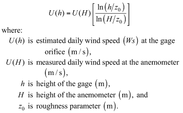
The estimated error in the total hydrologic budget was calculated as the residual of (inflows - outflows) - estimated change in storage (Winter, 1981) and represents the sum of errors in measurement or estimation of each water budget component and the sum of any unestimated components such as soil-moisture storage. Surface-water inflows were limited to small and periodic applications of irrigation water, and there were no significant outflows to surface water, pumping, or ground water. Insufficient information was available to estimate the soil-moisture storage independently.

Inflows

Inflows to the Wood River Wetland consisted of direct precipitation on the wetland, ground water, and applied water from flood irrigation. Because dikes and canals isolate the wetland, there are no significant surface-water inflows.

Precipitation

Daily precipitation data were acquired from the Agency Lake AgriMet station (AGKO), one in a network of satellite-based automated agricultural weather stations operated and maintained by the Bureau of Reclamation (Bureau of Reclamation, 2008a). The AGKO site is on the northwest shore of Agency Lake, 2.5 mi southwest of the Wood River Wetland (fig. 1, fig. 2). The precipitation data were used without adjustment for distance due to the close proximity of the weather station. The precipitation record was complete except for 10 days in March and April 2005. Missing values were estimated using precipitation records at the Klamath Falls, Oregon (KFLO) AgriMet station, about 32 mi south of the wetland (fig. 1) (Bureau of Reclamation, 2008b).

Precipitation at the AGKO site was measured using a 12-in. heated tipping-bucket rain and snow gage (Peter L. Palmer, Bureau of Reclamation, Boise, Idaho, written commun., 2008). The measurement of precipitation using rain gages is subject to errors from various sources (Smith, 1993, p. 3.18–3.19); however, Yang and others (1999, p. 491) stated that wind-induced gage undercatch of precipitation is the greatest source of bias. This is especially true for solid precipitation (snow and ice) measurements (Yang and others, 1998, p. 241). Unshielded rain gages, which includes the rain gage used at the AGKO site (Bureau of Reclamation, 2008c), are more susceptible to undercatch than shielded gages.

Yang and others (1998, p. 243) developed a set of best-fit regression equations to correct wind-induced undercatch for unshielded U.S. National Weather Service 8-in. standard precipitation gages based on the type of precipitation (rain, mixed, or snow) and the wind speed (Ws):

Rain R = exp (4.605 – 0.062 Ws^0.58)

Mixed R = 100.77 – 8.34 Ws

Snow R = exp (4.606 – 0.157 Ws^1.28)

where:

R is daily catch ratio (percent), and

Ws is daily wind speed at the gage height (m/s).

R, the daily catch ratio, represents the ratio of gage-measured precipitation influenced by undercatch due to wind to the expected gage-measured precipitation if there was no influence due to wind. These equations produce adjusted precipitation estimates that are similar to those obtained by Larson and Peck (1974, fig. 3, p. 859).

Because the precipitation gage and the anemometer (wind meter) at the AGKO site are not at the same height above land surface, a correction is needed to find the Ws at the gage height. The following Ws adjustment was used to find the Ws at the gage height based on the wind field profile (Benning and Yang, 2005, p. 278):

(2)

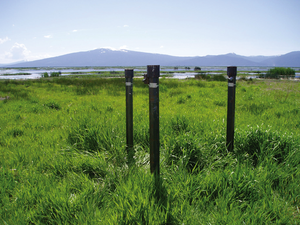
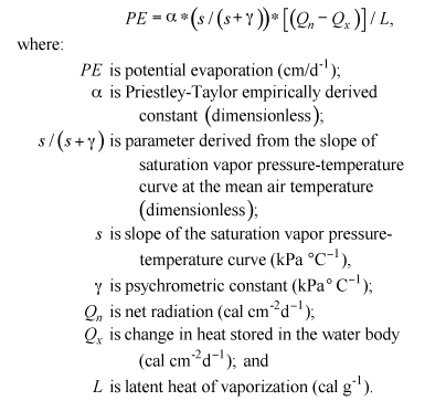
The measured daily wind speed at the anemometer, U(H), was recorded by the AGKO AgriMet station. The height of the rain gage, h, and anemometer at the AGKO AgriMet site, H, are 4.8 and 8.2 ft above land surface, respectively (Peter L. Palmer, Bureau of Reclamation, Boise, Idaho, written commun., 2008). The roughness parameter, z₀, was set to 0.01 m for a winter snow surface (December through March) and 0.03 m for short grass (April through November) based on values used by Yang and others (1998, p. 247) with seasonal adjustments appropriate for the Wood River Valley. The precipitation relations are applicable for wind speeds less than 6.5 m/s; therefore, adjusted wind speeds greater than 6.5 m/s (14.5 mi/h) were reset to 6.5 m/s to prevent overestimation of precipitation (Yang and others, 1998, p. 247; Benning and Yang, 2005, p. 278).

Daily precipitation adjusted for wind was calculated as the daily precipitation divided by R. Daily adjusted values of precipitation were summed to develop monthly estimates of inflow from precipitation. The median values of daily wind speed during individual events of rain, mixed precipitation, and snow were 6.1, 4.0, and 6.6 mi/h, respectively, for May 2003 through September 2005. The median values of estimated daily undercatch for individual events of rain, mixed precipitation, and snow were 11, 14, and 46 percent respectively during this period. Daily adjustment for wind-induced undercatch increases the gage-measured precipitation by about 19 percent on an annual basis.

Ground Water

Ground-water inflow to the Wood River Wetland takes place through numerous possible pathways: regional ground-water discharge through sediments, lateral ground-water seepage through dikes, and from direct discharge from flowing artesian wells.

Regional Discharge

The Wood River Wetland is adjacent to Upper Klamath and Agency Lakes, which are regional ground-water discharge areas (Illian, 1970; Leonard and Harris, 1974; Gannet and others, 2007, p. 46-47), and as such receives ground-water discharge from the upward movement of water from underlying aquifers. This is indicated by water levels in the five artesian wells (heads above land surface) and by the artesian water levels in the deepest piezometer (PZ-SU3, fig. 2). Preferential ground-water discharge also may occur through the natural internal streambeds, and the canal beds because of dredging associated with the construction of the canals to lower the water table by draining ground water from the wetland. During natural stream channel formation or canal construction, a significant clay confining layer (occasionally observed in soil cores, Rosenbaum and others, 1995, p. 33-34; Snyder and Morace, 1997, p. 7 and 26) may have been breached, providing significantly greater regional ground-water discharge than was calculated for the water budget. However, lack of data precluded inclusion of this type of discharge in the estimate of regional ground-water discharge.

Regional ground-water discharge was estimated using Darcy’s Law, which describes ground-water flow within a porous media (Darcy, 1856; Freeze and Cherry, 1979). Darcy’s law is expressed as: Q = AiK, where: Q is the volumetric flow [length³/time]; A is the cross-sectional area, perpendicular to the flow direction, through which flow occurs [length²]; i is the hydraulic gradient [dimensionless], and K is the hydraulic conductivity [length/time]. The law predicts that the volumetric flow of ground water is directly proportional to the hydraulic gradient and hydraulic conductivity of the media. The hydraulic gradient is the difference in the height of the water surface (that is, head difference) on either side of the dike divided by the length of porous media through which the head difference is distributed. Hydraulic conductivity is a measure of the ability of porous media to transmit water, with higher values indicating increased flow.

For diffuse regional ground-water discharge, the cross-sectional area perpendicular to ground-water flow was set equal to the area of each unit of the Wood River Wetland. Daily values of the hydraulic gradient were calculated as the daily head difference divided by the soil distance through which the head was transmitted. The head difference was calculated as the difference between the water level measured in the deep piezometer PZ-SU3 and the intermediate-depth piezometer PZ-SU2 (South Unit) as measured at least once every four months. Linear interpolation of these levels was used to calculate the daily head differences. The length through which the head difference was distributed was estimated as the distance between the centers of the open intervals for each piezometer (15 ft). Hydraulic conductivity was estimated to be 0.084 ft/d, which was the mean of slug tests performed on two piezometers: PZ-WRDK, on the dike adjacent to Wood River, and PZ-AGDK, on the dike adjacent to Agency Lake (fig. 2, table 2). The open intervals selected for these piezometers were representative of the undisturbed soils below the dikes. The lithology near the open intervals for these piezometers consists of hemic to sapric peat, silty clay with sand, and poorly sorted pumice sand and pebbles. The hydraulic conductivity estimate is in the high permeability range for clays, in the mid- to low range for peat, and in the low range for poorly sorted sands (Freeze and Cherry, 1979, p. 29; Wolff, 1982, p. 79-84; Fetter, 1994, p. 98). Daily values of regional ground-water discharge then were summed by month to create monthly estimates of inflow.

Seepage through Dikes

Water levels in the Wood River Wetland are lower than the elevation of surrounding surface-water bodies due to land subsidence and isolation from Agency Lake and the adjacent streams. This produces a head gradient conducive to seepage into the wetland, which was estimated using Darcy’s Law. Seepage was calculated daily and summarized monthly for the exterior dikes adjacent to a surface-water body including the Sevenmile Canal, Agency Lake, and Wood River dikes. Because sediments in the upper saturated zone consist of layers of peat, clay, and pumice (Snyder and Morace, 1997, p. 6–7, 25–26), flow through each was calculated separately using the thicknesses and hydraulic conductivity for each layer. The hydraulic conductivity of the clays, being several orders of magnitude less than that of pumice or peat, was excluded, as it was assumed to have a negligible contribution.

The cross-sectional area perpendicular to seepage through the dikes was calculated as the dike length multiplied by the vertical thickness of the pumice or peat layers. A thickness of 0.5 ft was selected for the pumice layer, and 7.5 ft for the peat soil layers, based on soil core data (Snyder and Morace, 1997, pl. 1). The thickness of the peat layers was augmented by the saturated area of the dike above the preexisting land surface as this material was primarily composed of dredged peat soils. The augmented thickness ranged from –0.8 to 3.2 ft depending on the water stages on either side of the dike.

The head difference was calculated as the daily difference between the elevation of Upper Klamath Lake (which adjoins Agency Lake) and water-surface elevation in the wetland measured at one of several staff gages. The stage of Upper Klamath Lake (USGS water-stage station 11507001 http://waterdata.usgs.gov/or/nwis/uv/?site_no=11507001) was selected because it is continually monitored and because the surface-water flow gradients between Upper Klamath and Agency Lakes and Agency Lake and its tributaries are so low that the monitored stage was assumed representative of all adjacent surface-water bodies. The elevation at the selected station for Upper Klamath Lake is actually a weighted mean elevation determined from three sites measured by the USGS. The distance through which the head difference was distributed was estimated as the distance across the base of the dikes using a detailed map derived from LiDAR (Light Detection And Ranging) data with a 1-m lateral resolution (see Haluska and Snyder [2007] for a description of the LiDAR data). The width of the dikes was set to 100 ft for days when wetland water level was above land surface at the base of the dikes and to 150 ft for days when water level was below land surface. Hydraulic conductivity for the pumice layer was set at 100 ft/d, based on literature values for sorted sand (Freeze and Cherry, 1979, p. 29; Wolff, 1982, p. 84; Fetter, 1994, p. 98). Hydraulic conductivity of the peat layer was set at 0.084 ft/d, the mean of slug tests performed on piezometers PZ-WRDK and PZ-AGDK because peat is the predominant lithology of the saturated zone in each piezometer.

Discharge from Artesian Wells

Five artesian wells in the Wood River Wetland continuously flow onto the land surface or directly to surface waters (fig. 2, table 3). Measurements of hydraulic head elevations during this and previous studies (Snyder and Morace, 1997; Gannett and others, 2007) ranged from 3.2 to 15.4 ft above land surface (table 3). Drilling records for these wells were unavailable, but soundings from four wells indicated depths ranging from 149 to 219 ft (Snyder and Morace 1997, p. 34; Gannett and others, 2007). Discharge rates from the artesian wells measured in a previous study (Snyder and Morace, 1997, p. 12) and as part of this study ranged from 2.6 to 20.2 gal/min (table 3). To develop monthly estimates of inflow from artesian wells, it was assumed that these wells discharged at a continuous rate over the period of the study equivalent to the measured values.

Applied Flood Irrigation

From 1999 to 2005, about 1,000 acre-ft of water was applied annually to the Wood River Wetland for irrigation, typically starting around September 15 and ending around October 31 (Bureau of Land Management, 2006, p. 4). The quantity of water applied to the wetland was not measured and instead was estimated by the approximate area and depth of inundation. During 2003, this water was transferred from the adjacent private tract located on the northwest side of the North Canal to the North Unit, and during 2004–05, the water was transferred from the Sevenmile Canal through the water control structure to the North Unit (fig. 2). To develop the water budget, this water was presumed to enter the wetland at a constant rate each year from September 15 through October 31 and was apportioned by month.

Outflows

Outflows from the Wood River Wetland included evaporation of open water and evapotranspiration from emergent vegetation. No major pumping of surface water took place during this study. No direct outflows from surface or ground water took place because of the low surface- and ground-water levels in the wetland relative to the area outside the wetland.

Daily estimates of evaporation and evapotranspiration for the North and South Units were made separately for open water and emergent vegetation as a function of the daily water-surface elevation, because the ratio of open water to emergent vegetation is a function of stage. A similar method was used in the Lower Klamath National Wildlife Refuge (fig. 1) by Risley and Gannett (2006, p. 5–10) using values for the land-cover types at the Wood River Wetland that represent open water and emergent vegetation. The ET in areas with open water and emergent vegetation was assumed to be dominated by the open-water component. The proportion of open water was determined daily using the stage–area relation previously derived (fig. 4). The remainder of the wetland area was assumed to be emergent vegetation.

Evaporation of Open Water

Pan-evaporation data often are used to estimate the rate of evaporation for open water. However, daily pan-evaporation data were unavailable for the upper Klamath River basin for the period of this study. Daily evaporation from the open-water areas was estimated as the potential evaporation calculated using the empirical Priestley-Taylor equation using daily observations of air temperature, water temperature, and solar radiation at a nearby weather station. The Priestley-Taylor equation (Winter and others, 1995, p. 984) is defined by the equation

(3)

The widely used Priestley-Taylor equation was selected because of its simple form, limited data requirements, and proven performance as a reasonable estimate of potential evaporation (Winter and others, 1995; Rosenberry and others, 2004). Values for the terms in the Priestley-Taylor equation were obtained as follows: the Priestley-Taylor empirically derived constant α was set equal to the commonly used value of 1.26, which has been determined to be representative for a fully saturated surface (Priestley and Taylor, 1972, p. 87; Winter and others, 1995, p. 991). The slope of the saturation vapor pressure-temperature curve s and the psychrometric constant γ were determined in a manner similar to Allen and others (2005, p. 10–11) using values of daily mean air temperature and elevation for the AGKO AgriMet site (Bureau of Reclamation, 2008a). The net radiation Q_n also was determined in a manner similar to Allen and others (2005, p. 11-25) using values of the observation date, daily global solar radiation, daily minimum and maximum air temperature, mean daily dewpoint temperature, elevation, and latitude for the AGKO AgriMet site (Bureau of Reclamation, 2008a) and a value of 0.08 (dimensionless) for the albedo of open water (Shuttleworth, 1993, p. 4.6). The change in heat stored in the water body Q_x also was determined in a manner similar to Shuttleworth (1993, p. 4.10, eqn. 4.2.20) using values of the density and specific heat of water, the daily change in water volume as determined using daily change in water depth for each unit of the Wood River Wetland, and the mean daily water temperature in a canal in an adjacent drained wetland at the AGKO AgriMet site (Bureau of Reclamation, 2008a), where water temperatures were assumed to be similar to those in the Wood River Wetland. The change in heat stored in the water body comprising the standing surface water in the North and South Units was nearly insignificant relative to the net radiation resulting from solar radiation. Ninety-five percent of the daily maximum magnitude values for the change in heat stored in the water body were equivalent to less than 4 percent of the daily net radiation magnitude. A value of 586 cal g^-1 was used for the latent heat of vaporization L (Allen and others, 2005, p. 9).

The daily temperature and global solar radiation records were complete except for 10 days in March and April 2005. Missing values were estimated using records at the Klamath Falls, Oregon (KFLO) AgriMet station (Bureau of Reclamation, 2008b). Because the open-water areas of the Wood River Wetland had water freely available for evaporation and were not water limited, it was assumed that the potential open-water evaporation calculated using the Priestley-Taylor equation was equal to the actual open-water evaporation. The daily rate of open-water evaporation was multiplied by the area representing the daily inundated area of the North and South Units to determine the volume of open-water evaporation in each unit on a daily basis and then summed to obtain monthly estimates.

Evapotranspiration from Emergent Vegetation

The evapotranspiration from the emergent vegetation component was estimated using a method described in Risley and Gannett (2006, p. 5–6). For the months of April–October, Risley and Gannett (2006) estimated evapotranspiration using results from a USFWS model based on the Priestley-Taylor evapotranspiration equation (Ronald R. Thomasson, U.S. Fish and Wildlife Service, Portland, Oregon, written commun., 2005). The model was calibrated using data from energy budget studies conducted at several sites in the Klamath Basin National Wildlife Refuge Complex (fig. 1) (Bidlake, 1997, 2000, 2002; Bidlake and Payne, 1998). Using a simulation period of 1961–90, the model predicted a median ET loss of 2.41 ft for April–October. Risley and Gannett (2006) used this value and the monthly reference ET rates estimated for the KFLO AgriMet station to represent ET losses for November–March. The annual ET loss for the emergent vegetation component was estimated to be 2.63 ft. Although the KFLO site is 32 mi south of the Wood River Wetland, comparison of the ET data from the AGKO and KFLO sites indicated that total ET for October 2003 through September 2005 differed by less than 5 percent, justifying their use for emergent vegetation ET rates. The monthly rate of evapotranspiration from emergent vegetation (table 4) was divided by the number of days in each month and then multiplied by the area representing the dry areas of the North and South Units to determine the volume of evapotranspiration in each unit on a daily basis. The daily volumes of evapotranspiration were then summed to obtain monthly estimates.

Changes in Storage

Standing Surface-Water Level and Volume

Daily changes in surface-water storage were determined using information on standing surface-water volume estimated using daily interpolated estimates of surface-water stage and a stage-volume relation developed from LiDAR data (Haluska and Snyder, 2007) (fig. 4). Measurements of surface-water stage consisted of nearly 60 sets of staff gage readings at three sites in the wetland (fig. 2) taken by BLM staff from May 19, 2003, to September 30, 2005. Each gaging site consisted of one to three staff gages to accommodate various surface-water levels. These gages were read with varying frequency, although many were less than 1 month apart. South Unit readings were infrequent during autumn through spring (September 2003 to February 2004, and November 2004 to May 2005). For the North Unit, readings were infrequent from November 2003 to February 2004 and from November 2004 to May 2005. Gage elevation (NGVD29) was determined by surveying instruments and the relation of staff gage readings to LiDAR imagery. Linear interpolation was used to estimate daily surface-water stage in the North and South Units for days with no observations. Although the lack of measurements for extended periods introduces uncertainty in the water budget, the interpolated results generally followed the water-level trend of adjacent Agency Lake.

The relation between the surface-water elevation and open-water area and standing water volume in the wetland were developed using LiDAR, photographic imagery, and a digital elevation model (DEM) (Haluska and Snyder, 2007). From these relations, lookup tables were prepared to calculate the inundated area and water volume in the wetland at various surface-water elevations. The lookup tables were used to determine the daily standing surface-water volume and the daily change in surface-water storage. Monthly change in surface-water storage was determined as the change of storage volume between the last day of the month and the last day of the previous month.

High water levels at the Wood River Wetland, South Unit (looking south southeast). Photograph taken by Kurt Carpenter, U.S. Geological Survey, July 2005.

Low water levels at the Wood River Wetland, North Unit (looking south southeast). Photograph taken by Kurt Carpenter, U.S. Geological Survey, July 2005.

Ground-Water Storage

The change in shallow ground-water volume in the saturated part of the subsurface represents a change in the volume of water stored in the wetland. The change in ground-water storage is equal to the change in saturated volume multiplied by the change in water or moisture content of the soil or subsurface material. The change in saturated volume is determined by the area and thickness of the ground-water level change. For ground-water level declines, the change in water content is equal to the specific yield of the subsurface material. Specific yield is a dimensionless number that is the ratio of the volume of water that a saturated porous medium will yield by gravity to the volume of the porous medium (Lohman and others, 1972, p. 12). For rising ground-water levels, the water content is dependent on the antecedent soil-moisture content due to the prior addition or subtraction of water in the unsaturated zone within the volume encompassed by the ground-water level rise. Increases in water content can occur through the infiltration of precipitation or applied water for irrigation and decreases in water content can occur through evapotranspiration from plants or soil. Because no data were collected regarding water content of the unsaturated zone, the change in water content of the unsaturated zone for ground-water level increases was assumed to be equal to the specific yield.

The monthly change in saturated volume of the subsurface materials was determined individually for the North and South Units. The change in the ground-water level for the shallowest well in each of the piezometer nests in each unit was interpolated on a daily basis. The ground-water level in each piezometer was assumed to be representative of the ground-water level throughout each wetland unit. The total volume of saturated soil, surface water, and air above the land or water surface between an arbitrary elevation (selected as the lowest land-surface elevation in the wetland 4,129.79 ft. NGVD29) and the daily interpolated ground-water level for the piezometers was calculated for each wetland unit by multiplying the area of each unit by the height of the ground-water above the datum (calculated as the difference of the ground-water level elevation and the arbitrary datum elevation). Depressions in the land surface of the wetland that are below the ground-water level elevation may be filled with either surface water or air. The part of the total volume containing surface water or air was determined by using the stage-volume relation for each unit for the corresponding elevation of ground-water and subtracted from the total volume. The remaining volume is the saturated wetland soil for each unit above the arbitrary datum for that day. The daily change in ground-water storage is a function of the daily change in saturated wetland soil volume and the specific yield of the soil. The monthly change in ground-water storage was calculated as the sum of the daily changes in saturated wetland soil volume for the month multiplied by the specific yield of the soil.

A value of specific yield for peat soils was selected for use because peat is the predominant lithology present by volume in the upper part of the subsurface at the Wood River Wetland (Snyder and Morace, 1997, pl. 1). Boelter (1965, p. 229–230) measured specific yield for moderately decomposed herbaceous peat and for well-decomposed peat, obtaining values of 0.15 and 0.10, respectively. The mean of these two values, 0.125, was selected for use in this study. Multiplying the monthly change in saturated volume for each wetland unit by a specific yield of 0.125 provides an estimate of the change in ground-water storage for each unit.

Soil-Moisture Storage

The change in soil-moisture storage in the unsaturated part of the subsurface represents a change in volume of water stored in the wetland. The change in soil-moisture storage often is assumed to be negligible over the course of a water year (water year is defined as October 1–September 30, and is identified by the year in which it ends), because depletion of soil-moisture storage is assumed to be equaled by replenishment through the infiltration of precipitation or other inflows. Although this assumption is generally valid when averaged over many years, variations during any single year could be significant. Soil-moisture storage can be calculated using information on soil-moisture content and volume of the unsaturated zone. The volume of the unsaturated zone can be estimated by using information on land surface from LiDAR data and by using the shallow ground-water levels recorded in the piezometers. No information was available on soil-moisture content; therefore, the change in soil moisture storage in the Wood River Wetland could not be directly calculated during this study.

Calculation of Standing Nutrient Masses

Nutrient dynamics in wetlands are the result of interactive relations among physical, chemical, climatic, and biologic components. Nutrient sinks include uptake by wetland plants, microbial denitrification, ammonia volatilization, and precipitation into insoluble compounds. Nutrient sources include ground water, wet and dry precipitation, waterfowl feces, nitrogen fixation, decomposition, and release of nutrients from sediments and decaying plant material. Quantifying each of these dynamic processes was beyond the scope of this study. However, it was possible to quantify the seasonal fluctuation of standing nutrient masses, which provided insights into the whole-system responses to dilution, evapoconcentration, and biogeochemical processes. Nutrient masses (in kilograms) were calculated for the North and South Units as the median nutrient concentration multiplied by the standing water volume estimated on each sampling date.