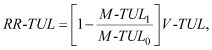
Methods


Tracer experiments were designed such that only one of the three variables of interest (wind forcing, Williamson River inflow, and lake elevation) was varied at one time. The wind forcing was varied in a realistic way by running 1-day simulations at 5-day intervals using continuous records of wind speed and direction measured between April 27 and September 30, 2008, while inflow and lake elevation were held constant. The 1-day time period was selected because the wind, although not constant, can be effectively characterized in terms of speed and direction over that time period; over longer time periods the wind variability can make it difficult to define a characteristic wind vector for the purposes of relating the wind forcing to the simulation results. Because continuous records of the wind forcing were used, each simulation also incorporates a realistic set of antecedent conditions. The entire April to September set of simulations was repeated for each value of inflow and lake elevation. The result was 384 tracer simulations (32 wind scenarios times 3 lake elevations times 4 values of Williamson River inflow). 


To quantify the results, two tracers were used to track the movement of water into and out of Tulana and Goose Bay and a third tracer was used to track the movement of water from the Williamson River into Tulana and Goose Bay. The amount of each of the first two tracers that left the Delta was calculated to determine a “total replacement rate” of water within each section of the Delta. The amount of the third tracer that entered the Delta was calculated to determine a “partial replacement rate” of water within each section of the Delta with water from the Williamson River. These total and partial replacement rates were used as dependent variables for building empirical regression models that used wind, lake elevation, and Williamson River inflow as independent variables.


Tracer Experiments


The hydrodynamic model of Upper Klamath and Agency Lakes was built on the UnTRIM computational core (Casulli and Cheng, 1992; Casulli, 1999; Casulli and Zanolli, 2002 and 2005). UnTRIM uses a semi-implicit, finite difference solution method to solve the governing equations for mass and momentum conservation on an orthogonal, unstructured, numerical grid. The advantage of this type of grid is that the size of the polygons that make up the grid vary over the domain in response to the local rate-of-change in the bathymetry, and it also allows for a shoreline-fitting boundary. The description of the process of calibrating and validating the three-dimensional UnTRIM model of Upper Klamath and Agency Lakes with data from 2005 and 2006 is described in Wood and others (2008). A one-layer version of the UnTRIM hydrodynamic model of the lake described in Wood and others (2008) was used to speed computation time. The use of a one-layer model removes the effects of water temperature (and therefore density) on the flow. These effects are important for understanding the transport of some water quality constituents, particularly dissolved oxygen and buoyant cyanobacteria (Wood and others, 2006, 2008). In this case, because the primary interest is the movement of water through the Delta, and the flow is expected to be well‑described by two dimensions, the benefit of being able to run many more simulations in the available time outweighs the loss of accuracy that occurs by using a one-layer model. The one‑layer model was recalibrated to velocity data collected with an acoustic Doppler current profiler at site ADCP1 in the middle of the trench (fig. 1) during 2007, using a grid that conformed to the shorelines of the lake at that time, prior to the breaching of the levees around Tulana.


The tracer simulations used for this report were generated using a numerical grid that incorporated the land inside the levees on both the Tulana and Goose Bay side of the Williamson River channel, as well as the channel itself up to approximately the location of the Modoc Point Road bridge (river kilometer 7.4). A Manning formulation was used for the bottom friction in these new areas of the grid. A Manning’s n of 0.026 was used within the channel to be consistent with a calibrated one-dimensional HEC-RAS model (Graham Matthews and Associates, 2001), and a Manning’s n of 0.05 was used in the Tulana and Goose Bay areas of the Delta, also consistent with Graham Matthews and Associates (2001). These bottom friction roughness coefficients also are consistent with those used in the MIKE-21 model that was used to develop the project design (Daraio and others, 2004).


The unstructured orthogonal grid used in the UnTRIM model is particularly well-suited to describing the small scale features and complicated boundaries associated with the Williamson River channel and the various levees remaining around the channel and the Delta. The elevations within the Delta were obtained from a composite of data interpolated to a grid with 100 ft horizontal spacing (L. Friend, ZCS Engineering, Inc., written commun., 2009). The grid was built from pre-project survey data in combination with the engineered design modifications for the project, then modified with additional surveys to collect data where the design elevations differed from the “as-built” elevations. These data were used to generate the bathymetry data in the new Williamson River and Delta areas of the grid, which were then merged into the existing grid for the rest of the lake (fig. 2).


The boundary conditions that are needed to run the model include the wind forcing at the surface and inflows at the Williamson and Wood Rivers, as well as the outflow at the Link River boundary, which, in the model, is the sum of the outflow at the Link River Dam and the irrigation withdrawals at the A-canal. The wind forcing was obtained from a spatial interpolation of 10-minute data from six meteorological sites (fig. 1), as described in Wood and others (2008). 


The number of model simulations was limited by practical considerations, and, consequently, three values of flow and lake elevation were considered. The maximum range in lake elevation relevant to this study is between full pool at 4,143.3 ft (1,262.9 m) and the elevation of the sills where the breaches in the levees were made at 4,139 ft (1,261.6 m). Within that range, values of 4,140.5, 4,141.5, and 4,142.5 ft (1,262.0, 1,262.3, and 1,262.6 m) were selected for model runs. The lake elevation constraint was implemented in the model simulations by specifying an initial lake elevation throughout the model domain at one of the three elevation values selected for model runs, and then specifying time‑invariant tributary inflows and outflows to the model domain. Evaporation and precipitation was set to zero, and the single outflow at the Link River was defined to be the sum of tributary inflows at the Williamson River and Wood River. In the model, the Wood River inflow includes the Sevenmile and Fourmile Canals that flow into Agency Lake. With these constraints, the simulated lake elevation remained constant, on average, through the length of the simulation; sub-daily variability on the order of several centimeters due to wind setup was superimposed on the long-term average. 


The values used for the flow in the Williamson River were 530, 883, 1,766, and 3,531 ft³/s, which correspond to 15, 25, 50, and 100 m³/s, respectively. These values span most of the large range in flows that could be expected in the Williamson River, but the mid-range values are more probable. In order to put these values into context, percentiles of the distribution of annual means and annual peak flows at the Williamson River USGS stream-gaging station (11502500) are provided in table 1. The inflows into Agency Lake at the Wood River, including flows from Sevenmile and Fourmile Canals, were calculated as 0.3 times the flows in the Williamson River. This was the May average of the ratio of the sum of the Wood, Sevenmile, and Fourmile flows to the Williamson River flow in 2004 (1 of 2 years in which all three inflows were recorded [Graham Matthews and Associates, unpub. data]). The month of May was relevant because the original reason for this study was to determine the connection between the Delta and the lakes during the annual spring migration of larvae out of spawning grounds. This ratio is, however, highly variable both within a single year, and in a given month between years, and the value of 0.3 is at the low end of the values measured throughout two consecutive years. Because of the variability of this ratio, sensitivity to this ratio was investigated and is reported with the results.


Three numerical tracers were used to track water leaving and entering the Tulana and Goose Bay sides of the Williamson River Delta. The first two tracers were initialized to a concentration of 10 (arbitrary units) at the start of each simulation in Tulana and Goose Bay, respectively, and zero elsewhere (fig. 3). The third tracer representing water in the Williamson River also was set to a concentration of 10 at the Williamson River upstream boundary, where all other tracers were set to a concentration of zero. Thus the third tracer tracked not only the water initially in the Williamson River channel, but also water that entered the model domain through the upstream Williamson River boundary at any time during the simulation. The total mass of each tracer within the boundaries of Tulana and Goose Bay was calculated at each time step. A 1-day total replacement rate (RR-TUL or RR-GB) for the tracers initialized within Tulana and Goose Bay was calculated at the end of the first day of each simulation as the decrease in the total mass of tracer within the Tulana and Goose Bay boundaries since the beginning of the simulation. The change in mass of tracer represents an equivalent change in the volume of the water that started the simulation within the boundaries of either side of the Delta, and can be expressed as either a volume rate of change (cubic meters per day or per second) or as a fraction of the entire volume of either side of the Delta (fraction of Tulana or Goose Bay volume per day). 


For example, the 1-day replacement rate in Tulana, in terms of cubic meters per day, was calculated as:


(1)


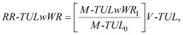
where M-TUL₀ and M-TUL₁ are the initial mass of the tracer within the boundaries of Tulana, and the mass of the tracer within the boundaries of Tulana at 1 day into the simulation, respectively. The volume of Tulana, V-TUL, is assumed invariant over the simulation. 


Similarly, a 1-day partial replacement rate (RR-TULwWR or RR-GBwWR) for the third tracer representing Williamson River water was calculated at the end of the 1-day simulation as the increase in the total mass of the third tracer within Tulana and Goose Bay since the start of the simulation. This provided a means of tracking how much of the water that replaced water initially in either Tulana or Goose Bay came from the Williamson River. For example, the partial replacement rate between Williamson River water and Tulana, in terms of cubic meters per day, was calculated as:


(2)


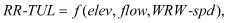
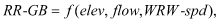
where M-TULwWR₁ is the mass of the Williamson River tracer within the boundaries of Tulana at the end of the 1-day simulation.


Multivariate Regressions


Multivariate regressions were developed for the total replacement rates in Tulana and Goose Bay, and for the partial replacement rates of water in Tulana and Goose Bay with water from the Williamson River. These regressions were based on the total and partial replacement rates calculated over 1 day as previously described and two different sets of independent variables in each case (variable definitions provided in table 2). Each set of independent variables incorporated lake elevation (elev), Williamson River inflow (flow), and a measure of wind strength (WRW-spd, -ew, or -ns) as recorded at the Williamson River West (WRW‑MET) meteorological station (USGS site 422807121572500) within the Williamson River Delta (fig. 1). The first set of independent variables incorporated the wind as speed only:


(3)


(4)


(5)


(6)


The second set of independent variables incorporated the wind as separate east-west and north-south components:


(7)


(8)


(9)


(10)


One value of each of the dependent variables was calculated for each tracer simulation, defined as starting at 5-day intervals between April 27 and September 29, 2008. The values of elev and flow were constants associated with each simulation. The value of wind speed or component magnitudes varied at the 10-minute observation interval over the simulation. These observations were condensed into a single explanatory variable for the multiple regression by taking the 75th percentile of the observations (subsampled at a 1-hour interval) of wind speed and the magnitude of the individual wind components. The use of the 75th percentile recognizes that peak winds may play a disproportionate role to their frequency of occurrence in accelerating the lake water. Each of the eight regressions were developed based on the calculations of total and partial replacement rates over 1 day (the first day of each simulation); the 75th percentile of the wind observations also was calculated for the first day of each simulation. 


The best functional form for each regression was determined by trial and error and by visual inspection of the residuals, as a function of the independent variables, as well as by using R² as a goodness-of-fit measure. The adjusted R² of the final regressions was the same as R² within two significant figures in all cases. The general form of regressions determined to be the “best” included the natural logarithm of lake elevation, wind speed and the magnitude of the east-west wind component as quadratic terms, and Williamson River inflow and the magnitude of the north-south wind component as linear terms. Multicollinearity of the independent variables was tested by examining the correlation matrix of the independent variables and assessing the values of variance inflation factors. All multivariate regression calculations were performed with SAS^® version 9.1 (SAS Institute, Inc., 2004). 


Following Wilks (1995), confidence intervals around the calculations of the dependent variable were estimated as the appropriate t-statistic (based on the number of degrees of freedom and the desired level of confidence) multiplied by the standard error of the estimate, which was computed as the square root of the mean squared residuals of the regression (RMSE). The RMSE values are reported with the results. 


First posted March 29, 2012