Groundwater Management Model


Water-Management Issues 


Water resources in the upper Klamath Basin are managed to achieve a variety of complex and interconnected purposes. Over the past decade, balancing the benefits of water for agriculture and for ecological needs has proven difficult. A series of Endangered Species Act biological opinions have required the Bureau of Reclamation’s Klamath Project to limit diversions from Upper Klamath Lake and the Klamath River (the principal sources of Project irrigation water) in order to protect habitat for endangered and threatened fish. Since 2001, Reclamation has been required to maintain elevations in Upper Klamath Lake to protect habitat for the endangered Lost River sucker (Deltistes luxatus) and shortnose sucker (Chasmistes brevirostris) (U.S. Fish and Wildlife Service, 2008), while simultaneously providing specified flows in the Klamath River to protect habitat for the coho salmon federally listed as threatened (National Marine Fisheries Service, 2010). This shift in water-management priorities resulted in substantial reductions in the amount of surface water diverted to the Project in 2001 and 2010, and has increased the likelihood that the Project will face water shortages in the future. 


In response to changing water-management priorities, Klamath Basin stakeholders have developed the proposed Klamath Basin Restoration Agreement (KBRA), which aims to restore historic fish habitat and populations in the upper Klamath Basin and establish reliable water supplies for agriculture (Klamath Basin Restoration Agreement, 2010). The KBRA includes a number of actions that substantially change water-resources management in the basin. Among those is the Water Resources Program (KBRA, Part IV), which establishes a permanent limitation on the amount of water that will be diverted from Upper Klamath Lake and the Klamath River. The proposed limitations on diversion, which are based on the forecast for net inflow to Upper Klamath Lake during the period April 1–September 30, vary from 330,000 acre-ft in low-inflow years to a maximum of 385,000 acre-ft in high-inflow years. An additional 48,000 acre-ft (low-inflow year) to 60,000 acre-ft (high-inflow year) will be diverted to the Lower Klamath Lake and Tule Lake National Wildlife Refuges, resulting in total annual maximum diversions of 378,000 to 445,000 acre-ft (KBRA, Section 15 and appendix E-1). The Water Resources Program also includes actions to improve streamflows and maintain the elevation of Upper Klamath Lake. The Agreement’s Water Use Retirement Program will rely on voluntary retirement of water rights or water uses to secure 30,000 acre-ft of water to increase inflow into Upper Klamath Lake (KBRA, Section 16), and the On-Project Plan includes criteria to ensure groundwater development does not have significant impacts on essential environmental flows (KBRA, Section 15). 


In contrast to the water management plan defined by the KBRA, historical water diversions to meet Project and refuge needs have actually been largest during dry years when inflows to Upper Klamath Lake tended to be smaller than average. This variability in diversions is primarily due to climate and reflects the increased demand for water in dry years. Prior to 2001, annual diversions from Upper Klamath Lake and the Klamath River (for both Klamath Project and refuge needs) ranged from about 320,000 to about 490,000 acre-ft (McFarland and others, 2005). A comparison of historical water diversion amounts to the maximum diversion amounts proposed in the KBRA indicates a reduction in the amount of water that can be diverted to the Project in dry years of as much as approximately 100,000 acre-ft.


Shifting water-management priorities are expected to create a sustained demand for groundwater to supplement surface-water supplies. Since 2001, groundwater use in the upper Klamath Basin has increased substantially, largely due to programs funded by Reclamation to augment the Klamath Irrigation Project’s surface-water supplies. These programs used a variety of methods in which farmers were compensated to use pumped groundwater as a substitute for surface water. In 2004, groundwater development associated with these programs increased groundwater use in the basin by about 50 percent over the estimated pumping in 2000, and more than doubled groundwater use in the area of the Bureau of Reclamation Klamath Project (Gannett and others, 2007). This sharp increase in pumping resulted in groundwater-level declines of 10 to 15 ft over much of the Project area. If groundwater use continues at the current level, the groundwater system will eventually achieve a new state of dynamic equilibrium. However, the spatial and temporal impact of this increased pumping on groundwater and surface water is unknown. The goal of the optimization model presented below is to assess the effect of sustained groundwater pumping on the complex and interconnected groundwater and surface-water system of the upper Klamath Basin in order to identify groundwater development strategies that result in acceptable impacts to groundwater and surface‑water resources.


Approach for Evaluating Future Groundwater Development


Groundwater development alternatives for the upper Klamath Basin were evaluated with the aid of coupled groundwater simulation and optimization models. A series of simulation-optimization models were developed to identify the key features and limitations of future groundwater development in the basin. The simulation-optimization models were designed to include the important hydrologic characteristics of groundwater development, such as the link between groundwater withdrawal and groundwater discharge to streams and lakes, the effect of increased pumping on existing groundwater users, and the impact of groundwater withdrawals on the Project’s drain system.


An important issue in testing future groundwater‑development scenarios is the impact of increased pumping on groundwater discharge that supports wildlife habitat, out-of-stream uses, and scenic flows. A substantial proportion of streamflow in the upper Klamath Basin consists of groundwater discharge, particularly in the late‑summer months when streamflow is needed to meet critical environmental needs for endangered and threatened fishes. The KBRA provides measures for defining and limiting the effects of groundwater pumping on environmental flows. The KBRA defines the “adverse impact” of pumping to mean a 6 percent or greater reduction in groundwater discharge to springs associated with Upper Klamath Lake, the Wood River and its tributaries, Spring Creek, the lower Williamson River, and the Klamath River and its tributaries. The KBRA further defines the measure of “adverse impact” to be only those effects of groundwater withdrawal that are caused by groundwater use within the Project. That is, the impact of groundwater pumping for the purpose of augmenting the Project’s surface-water supplies will be measured independently of the impact of all other stresses active in the basin. The simulation-optimization model presented below evaluates all groundwater-development scenarios to ensure that the impacts of groundwater withdrawal on environmental flows are within the limits defined in the KBRA.


A second issue to consider is the impact of groundwater development on existing groundwater users. OWRD determines whether wells have the potential to impair other groundwater users by causing substantial interference, a term that comprises many factors but generally refers to declines in groundwater levels that impair the ability of those with senior water rights to pump groundwater (Oregon Administrative Rules, 2011). Historically, substantial interference with other groundwater users has rarely been a problem in the upper Klamath Basin. However, due to the unprecedented increase in groundwater use since 2000, OWRD has been conditioning most new water right permits with water-level decline constraints. The conditions address short term (seasonal), year-to-year, and long term (multi-year) water-level declines. The simulation-optimization model has the capacity to test alternative groundwater-development strategies to ensure that drawdowns at a range of time scales are controlled and do not exceed limits consistent with OWRD standards. 


Finally, the analysis of groundwater-development scenarios must consider the impact of groundwater development on the operation of the Project. Subregions of the Project are hydrologically connected through the natural river network and the system of canals and drains. There is extensive re-circulation of drainage water throughout the Project, and the majority of on-farm irrigation inefficiencies are recycled through the use of drain water for irrigation (Burt and Freeman, 2003). Consequently, any groundwater discharge diverted from the drain system will reduce the amount of water available for irrigation. The Project’s infrastructure does not provide detailed measurement of the spatial and temporal variations of drain discharge or a detailed assessment of the spatial and temporal demand for drain water. Although there are no guidelines for defining excessive depletions in groundwater discharge to the Project’s drain system, the optimization model provides a flexible framework for evaluating a varied set of depletion limits. 


Simulation-Optimization Analysis


The groundwater flow model previously described in this report was coupled with techniques of constrained optimization to evaluate alternative groundwater‑development plans for the upper Klamath Basin. The example simulation‑optimization model described here consists of a mathematical formulation of groundwater-development goals (objective function) and a set of example constraints that limit those goals. The constraints are included to incorporate physical limitations of the groundwater system, along with other performance criteria, that must be honored. It should be noted that the example in this report does not incorporate climate (drought) cycles and off-project supplemental groundwater pumping, both of which will affect results. In addition, the example constraints may not represent those chosen by resource managers and water users in actual practice. Consequently, the example presented in this section is intended to demonstrate the concepts, functioning, and utility of the simulation-optimization model, and the numerical results are not intended to represent actual pumping targets. The simulation-optimization model:


• Evaluates groundwater/surface-water interactions for streams and lakes throughout the basin and ensures that the impacts of Klamath Project pumping on surface‑water resources are within prescribed limits. 

• Assesses the impact of Project pumping on groundwater levels and ensures that short- and long‑term drawdowns do not exceed limits designed to protect other groundwater users. 

• Identifies groundwater-development strategies for the Project that limit the impact of groundwater pumping on the Klamath Project drain system.

• Identifies groundwater-withdrawal strategies that support seasonal water demands for irrigation within the Project. 


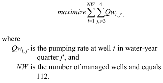
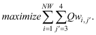
Mathematical Formulation of Objective and Constraints


The groundwater-optimization model applies the technique of constrained optimization, which uses mathematically formalized checks and balances to integrate complex water-management issues and quantitatively compare alternative groundwater-development plans. The use of optimization techniques allows consideration of an essentially limitless number of groundwater-development options. Formulation of the optimization model involves defining the model objective, decision variables, and a set of constraints. The optimization technique used in this study is sequential linear programming. The objective equation is linear; all constraint equations are linear or are linearized to allow solution using the sequential linear programming technique. Decision variables represent quarterly pumping at managed wells and are determined by the optimization model. The constraint set places limitations on drawdown and reduction in groundwater discharge to surface water and drains. The constraint set also places limitations on groundwater pumping to define seasonal demands on withdrawal rates and to define the allowable range of withdrawal for each well. 


Groundwater has been pumped at public-supply and irrigation wells throughout the upper Klamath Basin. The groundwater model described in this report includes about 1,000 wells that have been used during the period 1970–2004. The managed wells used in the optimization model are shown in figure 55A and represent the wells used in Reclamation’s groundwater acquisition program and pilot water bank. The optimization model calculates the pumping rates for the 112 managed wells; all other wells in the model are set to water-year 2000 pumping rates and are considered to be background stresses that contribute to the total stress acting on the groundwater system, but do not change from one simulation to the next.


The objective function of the optimization model was formulated to maximize the total pumping from the managed wells and is given by


(7)


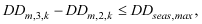
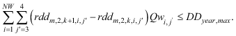
The objective function sums the quarterly pumping rate at each managed well over water-year quarters 3 and 4, which define the April–October irrigation season. The optimization model has 224 decision variables, which are the 3rd- and 4th-quarter pumping rates for each of the 112 managed wells. 


The analysis of groundwater-withdrawal strategies requires measures, known as constraints, to define the success or failure of alternative plans. The pumping rates identified by the simulation-optimization models were limited by a set of specified constraints on short- and long-term drawdowns; reduction in groundwater discharge to streams, lakes, and drains; seasonal demand for groundwater; and withdrawal rates for each well. The mathematical formulations of these constraints are defined in the following sections. The constraints used in a specific formulation of the optimization model, along with the constraint limits, varied among the different model applications. 


Groundwater withdrawal can have both short- and long-term impacts on groundwater levels. These range from the steep/large drawdown that generally occurs close to a withdrawal well and has a rapid onset and recovery, to the long-term drawdown that typically develops over a broad region after a period of sustained pumping. The optimization model included constraints on drawdown at 438 drawdown control sites shown in figure 55B. For each control location, three types of drawdown constraint—seasonal, year-to-year, and decadal—were defined. The numerical values used in this test case are broadly consistent with OWRD standards. The 2,500 ft model grid spacing limits the ability of the model to simulate pumping effects at finer spatial scales. As such, the model may underestimate large drawdowns very close to actively pumping wells. For this reason, seasonal‑drawdown constraints were set to limits slightly smaller than presently used for regulatory purposes. First, seasonal-drawdown constraints were defined to limit the lowering of the groundwater levels during the irrigation season (fig. 56).


      (8)


(9)


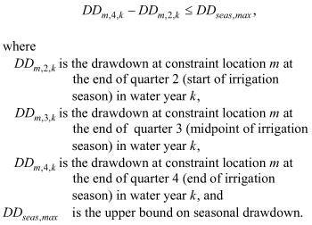
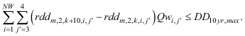
As illustrated in figure 56, seasonal drawdowns defined in equations 8 and 9 (DD_m,2,k, DD_m,3,k, and DD_m,4,k) are determined with respect to the water level calculated at the end of each quarter for the background simulation; that is, the simulation without managed pumping. The drawdowns defined in equations 8 and 9 are not the same as the change in groundwater levels calculated for the optimal pumping strategies from the second to the third (or second to fourth) water-year quarters. The seasonal drawdown constraints seek to limit only the drawdown that occurs due to the supplementary groundwater pumping evaluated in the optimization model, and therefore must take into account the variation in groundwater levels that occurs in response to the background stresses, as defined in equations 8 and 9 and presented in figure 56. The seasonal-drawdown limit was initially set to 20 ft. The impact of this limit was evaluated through sensitivity analysis.


A second, year-to-year drawdown constraint was defined to limit the “residual” drawdown remaining at the beginning of the irrigation season due to the previous year’s withdrawal.


(10)


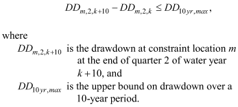
The year-to-year drawdown limit was initially set to 4 ft. A sensitivity analysis tested the impact of this constraint on model results.


A third, decadal drawdown constraint was included to limit the long-term drawdown resulting from sustained pumping over many years. Long-term drawdown was defined as the drawdown that occurs over a 10-year period.


(11)


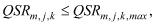
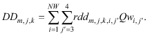
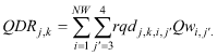
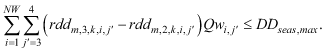
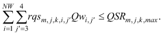
The long-term drawdown limit was set to 25 ft. Preliminary analyses indicated that the groundwater management model solution was not sensitive to this constraint for long-term drawdown limits greater than or equal to 10 feet. Therefore, this constraint limit remains unchanged in all model runs. 


Groundwater withdrawal is accompanied by declines in water levels that interact with surface water at a variety of temporal and spatial scales, potentially causing reductions in groundwater discharge to streams, lakes, and drains. Groundwater discharge to surface water is an important component of environmental flows that support wildlife habitat in the upper Klamath Basin, and groundwater discharge to drains supplies a component of the Project’s irrigation-water needs. Constraints on the depletion of groundwater discharge to streams and lakes required the depletion to be less than or equal to a specified maximum for 32 stream reaches throughout the basin and Upper Klamath Lake (fig. 55B). 


     (12)


(13)


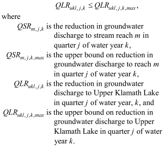
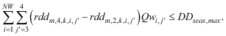
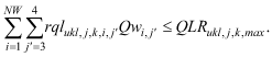
Constraints on the reduction in groundwater discharge to the Klamath River and Upper Klamath Lake and their tributaries were set to 6 percent of the baseline groundwater discharge, as specified in the KBRA, and were fixed at this value in all model runs. The base-case optimization analysis also includes a 6-percent depletion limit for the Lost River. Alternative formulations of the optimization model tested the impact of the Lost River constraint limit on model results. 


Similar constraints were defined to limit the reduction in groundwater discharge to drains (fig. 55B).


(14)


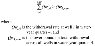
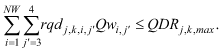
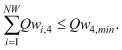
The constraints on the reduction in groundwater discharge to drains were initially set to 20 percent of the baseline discharge. The impact of these constraints was tested using sensitivity analysis. 


A demand constraint was included to evaluate the impact of seasonal demand for groundwater. The demand constraint imposes a minimum value on the sum of 4th quarter withdrawal rates from all wells. 


(15)


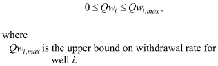
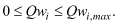
The base-case optimization model formulation does not include a demand constraint; a sensitivity analysis was performed to test the impact of this constraint. 


Finally, constraints on the minimum and maximum withdrawal rates for each well were defined as


(16)


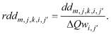
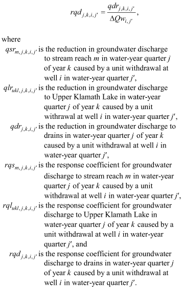
Upper bounds on withdrawal rates (maximum pumping rates) were estimated from water bank pumping records by dividing reported pumped volumes by the reporting period. Because this method assumes the volume was produced by continuous pumping over the reporting period, the estimated pumping rates are conservative. This is generally not a problem for this test case because estimated maximum pumping capacities were seldom reached in any of the solutions.


In summary, the groundwater management model was defined to maximize withdrawals from managed wells (equation 7), subject to constraints on drawdown (equations 8–11); reductions in groundwater discharge to streams, lakes, and drains (equations 12–14); water demand (equation 15); and withdrawal rates at managed wells (equation 16). Constraints on seasonal, year-to-year, and long-term drawdown were initially set to 20 ft, 4 ft, and 25 ft, respectively; the impacts of these limits on total withdrawal were evaluated through sensitivity analyses. Constraints on the depletion of groundwater discharge to the Klamath River and Upper Klamath Lake and its tributaries were fixed at 6 percent of baseline discharge values, as specified in the KBRA. Reductions in groundwater discharge to the Lost River were initially limited to 6 percent of baseline discharge values; alternative formulations tested the impact of varying the Lost River depletion limits. The depletion of groundwater discharge to drains within the Project was initially limited to 20 percent of baseline discharge, and was subsequently varied as part of a sensitivity analysis. Finally, the 4th quarter pumping demand constraint was set to zero in the base-case formulation, with alternative formulations tested in a sensitivity analysis. 


Response-Matrix Technique


The groundwater management model was formulated using the widely applied response-matrix technique. In this technique, unit solutions to the governing groundwater-flow equation (equation 1) are developed and linearly superposed to simulate the effect of groundwater withdrawal on drawdown and groundwater discharge. The responses are calculated only for the values of interest (drawdown and groundwater discharge to streams, lakes, and drains at constraint sites shown in figure 55) and only as a function of withdrawal at the managed wells shown in figure 55. The responses are compiled in a response matrix that is included as a set of constraints in the optimization model. The result is a compact version of the groundwater model that simulates the effect of managed withdrawal on water levels and groundwater discharge at those locations of critical interest to water-resources management. Detailed developments of the response-matrix technique can be found in Gorelick and others (1993) and Ahlfeld and Mulligan (2000). Literature reviews of simulation-optimization research can be found in Gorelick (1983), Yeh (1992), and Wagner (1995). Example applications that utilize optimization methods to address issues of groundwater development and groundwater–surface-water interactions include Barlow and Dickerman (2001), DeSimone and others (2002) and Granato and Barlow (2004). 


The first step in implementing the response‑matrix technique is calculation of the drawdown or groundwater‑discharge responses (at each of the constraint sites shown in fig. 55B) to simulated unit pumping rates at each of the wells in figure 55A. Calculation of the drawdown and discharge responses required 2NW + 1 simulations of the transient simulation model, where NW is the number of managed wells in the groundwater management model objective function (equation 7). In each of the 2NW simulations, the withdrawal rate for well i in water-year quarter j′ was increased by the unit pumping rate, ΔQw_i,j′; at the end of the quarterly stress period, the withdrawal rate for well i was returned to zero. The drawdown or reduction in groundwater discharge resulting from the unit withdrawal was determined by subtracting hydraulic heads (or groundwater discharge) simulated with the unit withdrawal rate from those simulated with background conditions in which the unit rate is inactive. The drawdown at constraint site m in quarter j of water year k, caused by a unit withdrawal at well i in quarter j′, is defined as dd_m,j,k,i,j′. Drawdown response coefficients, rdd_m,j,k,i,j′, are then defined as


(17)


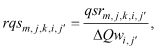
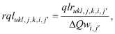
The characteristic drawdown responses are recorded for water‑year quarters j = 2,3,4 (the responses needed in the calculation of drawdown constraints) due to irrigation-season pumping ( j′= 3,4).


Similarly, the groundwater-discharge responses to a unit withdrawal at well i are defined as


(18)


(19)


(20)


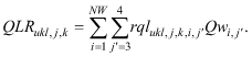
The response-matrix technique is based on the assumption that the numerical groundwater model is linear. In the case of a linear system, total drawdown and total reduction in groundwater discharge can be calculated using linear superposition


(21)


(22)


(23)


(24)


The response coefficients are the link between the simulation and optimization models of the upper Klamath Basin groundwater system. The response coefficients provide a compact version of the simulation model that calculates the effects of pumping on drawdown and groundwater discharge at constraint sites. The response coefficients are incorporated into the groundwater management model by substituting the right-hand sides of equations 21–24 into the left-hand sides of equations 8–14, to obtain the optimization model


(25)


(26)


(27)


(28)


(29)


(30)


(31)





(32)


(33)


(34)


Sequential Linear Programming


Complications can arise in the use of the response-matrix technique if the numerical model is nonlinear. The model of the upper Klamath Basin groundwater system has a number of recharge and discharge components that are simulated as piece-wise linear functions of the calculated hydraulic head. These boundary conditions can create nonlinear relations between hydraulic heads and discharges to or from a boundary. Examples of nonlinear relations important to the upper Klamath Basin model are those between hydraulic heads and groundwater discharge to streams, lakes, and drains found in the groundwater-discharge depletion constraints (equations 30–32). Because of these nonlinearities, the response coefficients can change as the simulated withdrawal conditions change. These types of nonlinearities have been handled in groundwater simulation-optimization problems by iterative methods that linearize the nonlinear head-dependent boundary equations (see, for example, Danskin and Gorelick, 1985; Danskin and Freckleton, 1989; Gorelick and others, 1993; Ahlfeld and Mulligan, 2000; Reichard and others, 2003; Ahlfeld and Baro-Montes, 2008). 


Sequential linear programming was used in this study to address the nonlinearities associated with head-dependent boundary conditions. Sequential linear programming solves a series of linear programming subproblems, each formulated using the response matrix technique. In each iteration of the method, the response coefficients are calculated using a unit rate added to the current managed flow rates; the current managed rates are derived from the previous iteration’s optimal withdrawal rates. The optimization problem (equations 25–34) is formulated and solved to provide updated managed withdrawal rates. The sequential process is continued until convergence is achieved. The convergence criterion used in this study is based on the objective function value (equation 25) and requires that the change in this value from iteration l to iteration l +1 be less than 0.05 percent. Two to eight iterations of the sequential linear programming method were required in the optimization results presented below. The model was formulated in each iteration of the sequential linear programming method using the response-matrix technique and was solved using the optimization software package LINDO (LINDO Systems, Inc., 2005). 


Transient Model Linked with Optimization


The coupled simulation-optimization model was designed to simulate dynamic equilibrium conditions in the same manner previously described for the example simulations. Formulated in this way, there is no net change in storage over the annual hydrologic cycle. The baseline model is intended to simulate average annual hydrologic conditions during the 1970 to 2004 transient calibration period. The optimized model simulates the same conditions as the baseline model, with the addition of increased groundwater pumping in the Project area. The spatial and temporal distribution of differences in hydraulic head and groundwater discharge between the baseline and optimized models are the basis by which the numerical model of the upper Klamath Basin groundwater system is incorporated into the groundwater management model. In the baseline dynamic-equilibrium model, simulated hydraulic head and groundwater discharge vary from quarter to quarter, but return to their initial state at the end of the annual cycle. In the optimized dynamic-equilibrium model, simulated head and discharge depart from the baseline conditions and reach a new state of dynamic equilibrium that is a function of the groundwater withdrawal identified by the optimization model. The dynamic-equilibrium model approach ensures that withdrawal strategies identified by the optimization model could be sustained without causing perpetual reductions in groundwater storage and discharge. The simulation-optimization models presented in this report were simulated with a twenty-year model horizon to allow the optimized withdrawal to reach a new state of dynamic equilibrium. 


Utilizing the dynamic-equilibrium model approach allows easy isolation of the impacts from supplemental pumping. The simulations do not, however, account for other external influences. Historical weather patterns in the upper Klamath Basin include decadal scale wet and dry cycles. Moreover, the background pumping in the example simulations does not include pumping historically associated with supplemental water rights in Oregon. These additional external influences, when incorporated into the simulation-optimization model, will affect the solution. Results presented in this report, therefore, are intended to demonstrate the utility of simulation-optimization model and should not be used for management purposes.


Evaluation of Selected Alternatives


Groundwater development in the upper Klamath Basin was evaluated with the aid of the coupled groundwater simulation-optimization model described in this report. Alternative management model formulations were examined to quantify relations between potential groundwater‑withdrawal rates and limits on groundwater drawdown, depletions in groundwater discharge, and groundwater demand. A varied set of management model applications were analyzed for alternative values of the drawdown, discharge, and demand constraints. Six sets of analyses were completed:


1. Base case. Drawdown limits defined as 20 ft for seasonal drawdown (equations 26 and 27), 4 ft for year-to-year drawdown (equation 28), and 25 ft for 10-year drawdown (equation 29); groundwater-discharge depletion constraints defined as 6 percent of baseline discharge for streams and lakes (equations 30 and 31); groundwater discharge depletion constraints defined as 20 percent of baseline discharge for drains (equation 32); no seasonal demand constraint. 

2. Analysis of the sensitivity of model results to the upper bound on changes to groundwater discharge to drains (equation 32).

3. Analysis of the sensitivity of model results to the upper bound on seasonal drawdown (equations 26 and 27).

4. Analysis of the sensitivity of model results to the upper bound on year-to-year drawdown (equation 28).

5. Analysis of the sensitivity of the model results to the 4th quarter (July–September) withdrawal demand (equation 33).

6. Analysis of the sensitivity of the model results to the upper bound on changes to groundwater discharge to the Lost River.


Base-Case Results


The results of the example base-case simulation‑optimization model are shown in figures 57–58. The optimization model provides 3rd and 4th quarter pumping rates for each of the managed wells shown in figure 55A. These represent the types of information, along with their spatial and temporal patterns, that are useful for practical implementation of a groundwater-development strategy. The solution of the sequential linear programming method gave a total withdrawal at managed wells of about 56,000 acre-ft during the April–September irrigation season, with quarterly rates of 198.3 ft³/s during April–June (3rd quarter) and 112.9 ft³/s during July–September (4th quarter). The managed pumping represents an increase of about 35 percent relative to pre-2001 pumping in the basin. Again, these figures do not reflect effects of drought cycles or nearby off-project supplemental pumping that will affect results. Figure 57 presents the optimal pumping by subregion and water-year quarter. Pumping by subregion ranges from approximately 1,000 acre-ft for the TID well group to approximately 29,000 acre-ft for the Klamath Valley well group. As a result of the drawdown and discharge restrictions imposed by the optimization model, there is significant unused pumping capacity in all but the Lower Klamath Lake well group. The wells of the TID group (fig. 55A) contribute the smallest amount to total pumping when measured as a percentage of a group’s pumping capacity (defined as the amount that could be withdrawn if all wells were pumped at their maximum rates). Of the total pumpage, 64 percent occurs as withdrawal during the 3rd quarter of the water year. By apportioning the majority of the pumping to the 3rd quarter, the optimization model is able to increase total pumping while meeting the year-to-year drawdown constraints. The ability of the groundwater system to accommodate increased 4th quarter pumping will be tested through sensitivity analysis.


Figures 58A and 58B show the distribution of pumping (geographically and with depth by model layer) for water-year quarters three and four respectively. The highest pumping rates are located in the southern Tule Lake and Klamath Valley areas. Eighty percent of the total pumping occurs at wells located in model layers 1 and 2 (denoted by TSY and TSO in table 1 and fig. 11); the remainder occurs at wells located in model layer 3 (denoted by TSV3 in table 1 and fig. 11). The difference in managed pumping with depth occurs despite there being approximately the same total capacity of the managed wells in layer 3 as there is in layers 1 and 2, and can be attributed in part to the lower storativity of the deeper zone of mixed sediments and volcanics. 


The results presented in figures 57 and 58 show a concentration of pumping in the Klamath Valley and southern Tule Lake areas. Water managers may wish to consider pumping patterns that redistribute some withdrawal to other areas. The optimization results can be analyzed to determine the trade-offs associated with increased (or decreased) pumping at selected wells. One measure of this trade-off is the reduced cost associated with each decision variable. Reduced cost is a local sensitivity that measures the change in the objective function resulting from a small change in the value of each pumping-rate decision variable (Gill and others, 1981; Ahlfeld and Mulligan, 2000). The reduced cost can be described alternatively as an ‘increased benefit,’ because if a pumping rate at a given location is at its upper bound, Qw_i,max, then the reduced cost is positive and represents the increase in the objective (equation 25) that would result from increasing Qw_i,max. In this case, the reduced cost measures the value of increased pumping capacity at location i. If Qw_i is greater than zero but less than Qw_i,max, the reduced cost is zero. If, however, Qw_i equals zero, the reduced cost is negative and represents the reduction in the objective (equation 25) that results from increasing Qw_i from zero. In this case, the reduced cost measures the penalty incurred when imposing a non-zero pumping rate at location i.


The reduced costs for the base-case optimization results are presented in figure 59. It can be seen that the greatest benefit would be obtained by increasing the capacity of a small number of wells found in the Klamath Valley, upper Lost River, and southern Tule Lake areas. All but one of the wells with reduced costs greater than 40 are located in model layers 1 and 2 (TSO and TSY in table 1 and fig. 11). Reduced costs that are negative indicate that increased pumping would be detrimental to the objective function. It can be seen in figure 59 that the greatest penalty would result from requiring pumping at wells with reduced costs less than –30 in the Klamath Valley, upper Lost River, northern Tule Lake, and southern Tule Lake areas. These wells are found in model layer 3 (TSV in table 1 and figure 11). There are also wells distributed throughout the Project area that have negative reduced costs between –15 and 0, indicating a relatively minor penalty if these wells are required to withdraw groundwater. These locations might be candidates for increased pumping if water managers required a different geographic distribution of pumping.


The locations of the constraints that limit withdrawal are shown in figure 60 and include 61 seasonal-drawdown constraints (38 in the 3rd quarter and 23 in the 4th quarter, figs. 60A and 60B), 12 year-to-year drawdown constraints (fig. 60C), groundwater discharge depletion constraints for two reaches of the Lost River (fig. 60A), and the drain discharge depletion constraint. All binding drawdown constraints occur in year 1 of the optimization model; the binding discharge constraints occur in year 20. The optimization results can be analyzed to identify the constraints that impose the greatest control on pumping. One way to do this is by examining the shadow price associated with each binding constraint. 


The shadow price is a local sensitivity that measures the marginal utility of relaxing a constraint, and it is defined as the amount by which the objective would change if the value of that constraint were changed by one unit (Hillier and Lieberman, 1980; Ahlfeld and Mulligan, 2000). The shadow price can be used to evaluate the potential gain in total withdrawal that results if a binding constraint is relaxed. Alternatively, water managers may wish to impose more restrictive limitations on drawdown or groundwater discharge. In this case, the shadow price can be used to estimate the reduction in total withdrawal associated with tighter constraint limits. 


The shadow prices for the binding seasonal-drawdown constraints range from about 0.2 to about 16 with an average of 2.7 (figs. 60A and 60B). The largest shadow prices for seasonal drawdown constraints are found in the southern Tule Lake and Klamath Valley areas. The magnitude of the shadow price for seasonal-drawdown constraints suggests there would be little improvement of the optimization objective if an individual constraint were relaxed. The results also indicate there would be little reduction in total pumping if a single constraint were tightened to impose a more restrictive drawdown limit. The optimization objective shows greater sensitivity to the binding year-to-year drawdown constraints and the binding discharge constraints. Shadow prices for the binding year-to-year drawdown constraints (fig. 60C) range from about 2 to about 170 (the average across all binding year‑to-year drawdown constraints is about 54), with the largest shadow prices found in the southern Tule Lake area. The shadow price for the binding discharge-to-drains constraint is about 1,050, and the average shadow price for the binding Lost River-discharge constraints is about 300. The shadow price values indicate that the greatest increase in total withdrawal would result from relaxing QDR_j,k,max, the upper bound on allowable depletion in groundwater discharge to drains, and the smallest decrease in total withdrawal would result from tightening the seasonal-drawdown constraint, DD_seas,max. It should be noted that the large number of binding seasonal drawdown constraints could result in a significant increase (decrease) in total pumping if the seasonal drawdown limit, DD_seas,max, is uniformly increased (decreased) across all constraint locations. The sensitivities to drain discharge, seasonal drawdown, year-to-year drawdown, seasonal water demand, and Lost River-discharge constraint limits are evaluated the following sections. 


It is important to note that the groundwater-discharge depletion constraints related to environmental flows in streams and lakes (equations 30 and 31) were not limiting. As described earlier in this report, the impact of pumping will depend on the rate of pumping, the hydraulic properties of the aquifer, and the proximity to hydrologic boundaries, such as streams, lakes, drains, and ET surfaces. The managed wells are found in an area with an extensive network of agricultural drains, shallow groundwater (with associated evapotranspiration losses), Lower Klamath Lake, the Tule Lake sumps, and the Lost River. The water pumped by the managed wells comes primarily from these boundaries. The largest impact of the increased pumping to environmentally sensitive areas was determined to be along a reach of the Klamath River between Keno and John C. Boyle Reservoirs. The simulated effect of the optimized pumping is to decrease groundwater discharge to this reach by about 0.13 percent, which is well within the 6-percent limit defined in the KBRA and required by the optimization model formulation. 


Vary Limit of Groundwater Discharge Constraints for Drains


The shadow prices presented in figures 60A–60C measure the local sensitivity of the objective to changes in the value of a binding constraint’s right hand side. It is useful to test the impact of larger changes in constraint bounds on the objective value. The first set of analyses evaluates the sensitivities of the optimal groundwater withdrawals to changes in the constraint controlling groundwater discharge to drains (equation 32), which was set to 20 percent of the baseline discharge in the base-case analysis. The allowable reduction in groundwater discharge to drains was varied from 10 percent to 40 percent of baseline conditions. As shown in figure 61 and table 4, total groundwater withdrawal varies from about 33,000 acre-ft for a discharge-depletion limit of 10 percent to about 77,000 acre-ft for a limit of 40 percent and higher. As the drain-discharge depletion constraint is increased from the 10-percent limit, the total withdrawal increases in an approximately linear manner until the constraint limit reaches 30 percent. In other words, the marginal utility of increasing QDR_j,k,maxis approximately the same for values of QDR_j,k,maxas much as 30 percent. At a constraint limit of 40 percent and beyond, however, the discharge depletion constraint for drains is no longer binding and there is no utility in further relaxing this constraint, as indicated by the shadow price of 0 (fig. 61).


The tradeoff curve presented in figure 61 highlights the importance of understanding the spatial and temporal patterns of drain-water discharge and groundwater pumping within the Project. The optimization model indicates the total withdrawal could vary by approximately 44,000 acre-ft depending on the limit imposed on groundwater discharge to drains (with all other constraints fixed at their base-case limits). Improved information about the patterns of drain-water discharge and demand would reduce the uncertainty associated with the value of this constraint and would provide a better understanding of the potential for groundwater development. 


Vary Limit of Seasonal Drawdown Constraints


The second set of analyses was developed to evaluate the sensitivities of the optimal groundwater withdrawals to changes in the seasonal-drawdown limit, which is designed to prevent excessive declines in groundwater levels over the irrigation season. In the base-case analysis, the seasonal‑drawdown constraints had the smallest shadow prices, indicating the model solution was least sensitive to these limits. The seasonal-drawdown limit found in equations 26 and 27, DD_seas,max, was varied from 10 ft to 30 ft. The results are presented in figure 62 and table 5. Total groundwater withdrawal varied from about 52,000 acre-ft with the seasonal-drawdown limit of 10 ft, to about 57,000 acre-ft for a seasonal drawdown limit of 30 ft. As shown in figure 62, an increase in DD_seas,max from 20 ft to 25 ft increases total pumping by about 1 percent, which is consistent with the small shadow price associated with binding seasonal‑drawdown constraints in the base-case solution (figs. 60A and 60B). Likewise, a reduction in DD_seas,max from 20 ft to 15 ft has little impact on total withdrawal. However, the effect of reducing the seasonal drawdown limit shows a nonlinear pattern. Reducing the limit from 20 ft to 15 ft causes a reduction in total withdrawal of about 1,000 acre-ft. If the seasonal‑drawdown constraint is further reduced to 10 ft, then the total withdrawal is reduced by an additional 3,000 acre-ft. The nonlinear pattern of this tradeoff curve is also reflected in the shadow prices, which increase in magnitude as the seasonal-drawdown constraint decreases. As the seasonal‑drawdown constraint is tightened, there is also a shift in the type and location of binding constraints. For a seasonal‑drawdown limit of 10 ft, the number of binding seasonal-drawdown constraints increases to 147 and the year‑to-year drawdown constraints no longer influence the solution. 


Vary Limits of Year-to-Year Drawdown Constraints


The third sensitivity analysis tests the impact of changing the year-to-year drawdown limit on the optimization results. The year-to-year drawdown constraint (equation 28) limits the residual drawdown at the beginning of an irrigation season due to pumping that occurred in previous years. In the base-case optimization model, the year-to-year drawdown constraint was set to 4 ft. The optimal solution identified 12 locations with binding year-to-year drawdown constraints, with an average shadow price of 54 (fig. 60C). In this analysis, the year-to‑year drawdown limit was varied from 2 ft to 8 ft. The results are presented in figure 63 and table 6. The results reveal a mildly nonlinear relation between total withdrawal and the year‑to‑year drawdown limit. Total withdrawal varies from about 53,000 acre-ft for a year-to-year drawdown limit of 2 ft to about 57,000 acre-ft for a limit of 8 ft. 


Vary Limits of Constraint for Seasonal Water Demand


The fourth sensitivity analysis tests the impact of the seasonal-demand constraint (equation 33). This constraint requires a minimum withdrawal rate from all managed wells during the 4th quarter of the water year. The base-case optimization model identifies 56,000 acre-ft of withdrawal, with about 20,000 acre-ft (36 percent) pumped in the 4th quarter of the water year (figs. 57 and 58B). In the fourth set of analyses, the minimum total withdrawal from all wells in the 4th quarter was systematically increased from approximately 23,000 acre-ft to approximately 45,000 acre-ft in increments of approximately 4,500 acre-ft (fig. 64 and table 7). For a 4th quarter demand of 23,000 acre-ft, total withdrawal decreased by about 100 acre-ft , and for a demand of 41,000 acre-ft, total withdrawal decreased by about 7,000 acre-ft. When demand was increased to 45,000 acre-ft, the model was infeasible because it was unable to identify a distribution of 4th quarter withdrawal rates that total 45,000 acre-ft while simultaneously limiting seasonal drawdown to 20 ft and year-to-year drawdown to 4 ft. 


Vary Limit of Groundwater Discharge Constraints for the Lost River


The Lost River is a source of irrigation water in the upper Lost River subbasin. The analyses presented thus far impose a 6-percent limit on the depletion in groundwater discharge to the Lost River. This sensitivity analysis evaluates the impact of increasing this limit to allow a greater reduction in groundwater discharge to the Lost River. The allowable reduction in groundwater discharge to the Lost River was varied from the base-case limit of 6 percent to 50 percent (fig. 65 and table 8). When the limit is increased to 15 percent, total pumping is about 58,000 acre-ft, which is approximately a 2-percent increase from the base case. For a 50-percent limit, total withdrawal is about 60,000 acre-ft. 


First posted May 5, 2012