SIMPLIFIED COST MODELS FOR PREFEASIBILITY
MINERAL EVALUATIONS
-
By Thomas W. Camm
-
Mining engineer, Western Field Operations Center, U.S. Bureau of Mines, Spokane, WA.
ABSTRACT
In this U.S. Bureau of Mines report, mine and mill cost models are presented to make quick estimates of the cost to develop mineral deposits in the desert region of the Southwest United States. Regression analysis was used to generate capital and operating cost equations for each model in the form Y = AX', where Y is the cost estimated and X is the assumed daily capacity in short tons. A and B are constants determined by the regression analysis. Each is broken down into 11 subcategories to facilitate escalation of costs for inflation and to increase their versatility in economic evaluation work.
This report contains 2 open pit models, 6 underground mine models, 11 mill models, and cost equations for access roads, power lines, and tailings ponds. In addition, adjustment factors for variation in haulage distances are provided for open pit models and variation in mining depths for underground models.
INTRODUCTION
The format for the cost models in this handbook was developed at the Bureau's Western Field Operations Center (WFOC), Spokane, WA, for studies of known and undiscovered resources on Federal lands (1-2). These studies required development of a methodology to estimate operating and capital costs for a mineral deposit given its tonnage, grade, and depth. The resulting models are summarized in this publication.
The format for these models was adapted from the Bureau's Cost Estimating System (CES) Handbook (3-4). CES is based on three regression equations (labor, supplies, and equipment) for each individual unit process. These equations are further expanded for more detailed breakdowns (steel, fuel and tube, explosives, etc.) by applying percentages to each of the three regression equations. To perform a complete analysis using CES, a thorough design scheme for the deposit must be performed to supply all the design parameters necessary for CES. This is the normal approach taken for Minerals Availability type studies performed by the Bureau. However, for policy analysis work where specific data on each deposit are not available, or where a regional analysis is necessary, the requirement for detailed engineering design parameters makes CES inappropriate.
A new modeling approach was developed to address this spec application. The models are ideal for making quick cost estimates where specific design parameters are unavailable. The modeling approach used in this simplified methodology is particularly well suited for this circumstance. Users in the Bureau's Resource Evaluation and Policy Analysis divisions, professionals outside the Bureau performing similar evaluations, and those who need a quick cost estimate for a mineral deposit will find the approach of this simplified method particularly useful. The key benefits of the method are: demands less engineering background of user, ease of applying escalation factors, versatility in applications to a variety of deposit types, will occupy significantly less space on a computer than alternative systems, and the limited design parameters necessary to conduct a cost estimate. The cost derived using these models should be considered a prefeasibility type estimate.
These models were originally developed to evaluate the California Desert Conservation Area (CDCA) in southern California. They. are also applicable for any similar type operation in a desert region in the Southwest United States. Costs should be adjusted for application to regions with more severe weather (requiring more substantial buildings), more vegetation (requiring more clearing costs), or steeper topography.
In addition to this publication, these cost models have been incorporated in PREVAL - Prefeasibility Software Program for Evaluating Mineral Deposits by R. Craig Smith, physical scientist, Intermountain Field Operations Center, Denver, CO (5).
ACKNOWLEDGMENTS
The author thanks the following colleagues (all at WFOC) for assistance in costing individual capacity scenarios for several of the models: David A. Benjamin, David S. Lindsey, James M. Spear, Scott A. Stebbins, and Nicholas Wetzel.
METHODOLOGY
Models were developed using a variety of sources, with the intent of providing the most accurate representation of costs available for each model. Costs for several operations at varying tonnages were estimated. Wherever feasible, capacity scenario was based on actual operations. Site information available included flowsheets, equipment
Italic numbers in parentheses refer to items in the list of references preceding the appendixes at the end of this report.
lists, and manning charts. This information was augmented by data from cost handbooks and references (3-4, 6-10) which contained individual components cost and use rate. Additionally, cost models developed at WFOC for previous studies were adapted for certain cases where feasible (1-2).
Following determination of representative daily capacities for each model and gathering of pertinent data, capital and operating costs were generated for each capacity. These costs were summarized in the following categories: labor, equipment, steel, lumber, fuel, tube, explosives, tires, construction materials, reagents, and electricity. In addition, a separate category for sales tax-based on a California rate of 6%-was included. Sales tax was applied to all cost categories except labor, fuel, tube, and electricity. A total cost equation was also included for each model, for users who do not require a cost breakdown into each of the individual categories, but only an overall cost estimate.
Regression analysis was used to generate capital and operating cost equations for each model in the form Y = AXB, where Y is the cost estimated and X is the assumed capacity in short tons per day (st/d). A and B are constants determined by the regression analysis. Costs of mining and other industrial operations historically fit this equation form, and this is consistent with the format of CES cost equations. Equations for each category listed above that were appropriate to the model were calculated in this form. Having the costs expressed in these categories facilitates escalation of costs for inflation and increases their versatility in economic evaluation work.
A summary of each of the total cost equations, with corresponding square of the correlation coefficient (r2) and number of observations, is included in appendix A.
Because of their nature some cost categories have not been covered by the models. They, therefore, must be considered separately. The most important of these are: preproduction exploration, permitting, environmental studies, State and Federal taxes (except State sales tax on specified cost items), corporate overhead, site reclamation, concentrate transportation, and smelting and refining charges (except where noted for models that include production of gold-silver dote).
CAPITAL COSTS
Capital costs are based on actual equipment list prices in most cases. An additional cost of 7.5% is applied to all equipment purchase costs for freight. Equipment lists for the open pit models were based on actual operations, adjusted to fit the generic nature of the handbook. Underground capital costs were determined by the amount of development necessary for an underground mine of the size and type under consideration to begin operating at design capacity. A cost factoring method similar to the approach developed by Mular (7) was used for many of the mill models. Working capital, based on 2 months of operating costs, was included in the capital cost of each mine and mill model. Working capital covers the cost of meeting operating costs in the initial stages of production, before revenue is generated from the first shipments of product (concentrates or dote). This value can vary from
2 to 6 months. Engineering and construction management fees are also included in the capital cost models.
OPERATING COSTS
Operating costs are based on daily capacity (st/d) and are expressed in dollars per short ton ($/st). The open pit models are based on X = st/d of ore and waste moved. This allows for the wide variability in stripping ratios found among different open pit operations. All the underground models are based on st/d of production, and costs are in $/st. Mill models are based on mill feed (st/d) and the costs are in $/st mill feed.
ADJUSTMENT FACTORS
Adjustment factors are included for mining models to reflect variability among different ore deposits. Open pit models have a base-case cost equation for a specified haulage distance calculated in a manner discussed in the open-pit section. In addition to the base-case equations, another set of equations are provided with a factor for varying haulage distances. These factors are explained fully in the open pit section and in appendix B.
Underground mining models are also established using a base case. In this instance, the basic assumption for the underground mining models is an adit entry to the mine. To allow for the variability in access depth common to underground mining, depth adjustment factors are provided at the beginning of the underground section. These factors are to be applied to the base-case equations where access to the ore body is by shaft entry. An explanation of the factors, and a table summarizing them for application to all underground models, is found at the beginning of the underground mining section.
INFRASTRUCTURE
Costs for powerlines and access roads are included in the infrastructure section. These costs are to be applied where a powerline needs to be constructed to supply power to the site, and where access roads must be constructed to the site.
For mills requiring tailings ponds, cost equations for tailings pond construction are provided in the beginning section of the mill models.
MINE DILUTION AND RECOVERY FACTORS
Mining seldom recovers all resource present in an ore deposit. The amount of ore actually extracted from a deposit is referred to as the recovery factor and is expressed as a percent. In addition, a certain amount of waste is usually mixed in with the ore during mining. This waste mixed in as ore is called dilution and is usually expressed as a dilution factor (in %). Both recovery and dilution vary with each ore body, but tend to be within a similar range for each mining method. Table 1 summarizes the assumed dilution and recovery factors used for the mine models and reflects values commonly encountered when these mining methods are applied.
|
Table 1. Mine dilution and recovery factors |
|
Mining method |
Dilution |
Recovery |
|
|
factor, % |
factor, % |
|
Open pit |
5 |
90 |
|
Block caving . . . . . . . . |
15 |
95 |
|
Cut-and-fill |
5 |
85 |
|
Room-and-pillar . . . . . . |
5 |
185 |
|
Shrinkage |
10 |
90 |
|
Sublevel longhole . . . . . |
15 |
85 |
|
Vertical crater retreat . . |
10 |
90 |
|
'Assumes pillar extraction. |
|
|
MINE LIFE
Given a known ore reserve tonnage, the life and daily capacity for a typical mining operation can be determined. Taylor (11) developed an equation commonly used in prefeasibility studies to determine mine life, known as Taylor's rule (equation 3). Based on this rule, the basic equation for C (capacity of ore production in st/d) is:
-
(1)
-
-
where L = mine life in years,
-
T = total tonnage (in st) of ore to be mined,
dpy = operating days/yr.
To find T, recovery and dilution factors (table 1) are applied to the total amount of ore in the deposit:
(2)
-
where rt = total deposit reserve tonnage in st,
-
rf = recovery factor for the particular mining method from table 1,
df = dilution factor from table 1.
Substituting for L using Taylor's rule (11):
(3)
We can determine the daily mining capacity with either equation 4 or 5 below, depending on whether the operating days per year are 350 or 260 (equivalent to operating 7 d/wk or 5 d/wk, respectively).
(4)
(5)
where C1 = mine capacity in st/d for 350 d/yr
(7 d/wk),
C2 = mine capacity in st/d for 260 d/yr
(5 d/wk).
COST UPDATING
All costs are based on average 1989 dollars. Cost categories correspond to the Bureau's CES Handbook, with some minor adjustments. There is only one labor index, and the fuel and tube categories are separate in the models developed for this publication. Two categories, electricity and chemical reagents, are included that are not found in CES. Cost indexes used for the models are summarized for the years 1967-1989 in table 1` Included in the table is the Marshall & Swift index (12-14) for escalating capital costs of mining and milling operations.
To update costs for a given equation, divide the index for the specified date by the base year cost index (1989), and multiply the cost equation by this factor. For example, to update the fuel operating cost for the small open pit model to 1990 dollars (equation 6), first look up the escalation index for fuel and lube in 1990 = 74.8. By then looking in table 2, determine the base year index is 61.2. Divide the 1990 index by the base year index, and multiply by the cost equation from table 6. Assume a 10,000 st/d operation:
(6)
|
Table 2-Historical cost
Indexes (1) |
|
Year- |
Mining |
Equipment |
Bits |
Timber |
Fuel |
Explosives |
Tires |
Construction |
Electricity |
Chemical |
Mining, |
| Code (2) |
labor |
and repair |
and |
and |
and |
|
And |
material |
|
reagents |
milling |
| |
|
parts |
steel |
lumber |
lube |
|
rubber |
|
|
|
|
| |
C-1 (3) |
|
|
|
|
|
|
Bldg. Cost(4) |
|
|
M&S
(5) |
|
|
|
|
|
|
|
|
|
|
|
|
|
| 1967 .. |
3.19 |
29.1 |
29.5 |
32.2 |
13.1 |
33.5 |
36.8 |
100.0 |
21.1 |
28.4 |
263.5 |
| 1968 .. |
3.35 |
30.7 |
30.1 |
37.8 |
12.9 |
34.2 |
37.8 |
127.0 |
21.3 |
28.6 |
273.2 |
| 1969 .. |
3.60 |
32.1 |
31.6 |
2.3 |
13.1 |
35.0 |
36.2 |
108.0 |
21.6 |
28.4 |
284.5 |
| 1970 .. |
3.85 |
33.7 |
34.0 |
36.6 |
13.3 |
35.7 |
38.8 |
109.0 |
22.5 |
28.6 |
302.6 |
| 1971 .. |
4.06 |
35.4 |
35.9 |
43.8 |
14.1 |
37.9 |
40.6 |
133.0 |
24.8 |
28.9 |
321.1 |
| 1972 .. |
4.44 |
36.6 |
37.9 |
51.3 |
14.3 |
38.5 |
41.0 |
151.0 |
26.2 |
28.7 |
331.8 |
| 1973 .. |
4.75 |
38.0 |
40.2 |
66.0 |
16.9 |
40.2 |
42.6 |
154.0 |
28.0 |
29.3 |
342.9 |
| 1974 .. |
5.23 |
44.3 |
52.7 |
66.6 |
29.3 |
50.2 |
52.1 |
167.0 |
36.4 |
43.0 |
394.3 |
| 1975 .. |
5.95 |
53.8 |
59.3 |
61.9 |
33.8 |
59.5 |
57.2 |
186.3 |
44.3 |
58.7 |
451.2 |
| 1976 .. |
6.46 |
57.8 |
63.7 |
75.0 |
36.3 |
62.6 |
63.6 |
205.5 |
47.9 |
62.2 |
482.9 |
| 1977 .. |
6.94 |
62.1 |
68.0 |
89.0 |
40.5 |
64.9 |
66.9 |
237.7 |
54.3 |
63.5 |
520.8 |
| 1978 .. |
7.67 |
67.7 |
74.8 |
103.7 |
42.2 |
69.8 |
70.7 |
247.7 |
59.1 |
64.0 |
564.7 |
| 1979 .. |
8.49 |
74.5 |
83.6 |
114.0 |
58.4 |
75.5 |
80.9 |
269.3 |
64.5 |
74.9 |
619.2 |
| 1980 .. |
9.17 |
84.2 |
90.0 |
104.9 |
88.6 |
84.0 |
92.1 |
287.7 |
77.8 |
91.9 |
683.5 |
| 1981 .. |
10.04 |
93.3 |
98.5 |
104.6 |
105.9 |
96.7 |
99.5 |
310.3 |
89.2 |
103.1 |
740.2 |
| 1982 .. |
10.77 |
100.0 |
100.0 |
100.0 |
100.0 |
100.0 |
100.0 |
330.1 |
100.0 |
100.0 |
783.8 |
| 1983 .. |
11.28 |
102.3 |
101.3 |
113.5 |
89.9 |
101.1 |
95.7 |
352.9 |
103.1 |
97.3 |
799.3 |
| 1984 .. |
11.63 |
103.8 |
105.3 |
112.5 |
87.4 |
103.6 |
93.4 |
357.9 |
108.4 |
96.8 |
816.5 |
| 1985 .. |
11.98 |
105.4 |
104.8 |
109.6 |
83.2 |
105.0 |
90.5 |
358.2 |
112.8 |
96.0 |
822.6 |
| 1986 .. |
12.46 |
106.7 |
101.1 |
110.5 |
53.2 |
103.6 |
88.0 |
367.3 |
114.5 |
91.5 |
827.1 |
| 1987 .. |
12.52 |
108.9 |
104.6 |
118.2 |
56.8 |
107.3 |
87.7 |
375.6 |
111.9 |
95.5 |
837.1 |
| 1988 .. |
12.69 |
111.8 |
115.7 |
122.1 |
53.9 |
108.8 |
92.4 |
384.6 |
112.8 |
106.8 |
870.0 |
| 1989 .. |
13.14 |
117.2 |
119.1 |
125.7 |
61.2 |
117.6 |
96.3 |
390.7 |
116.2 |
114.8 |
911.9 |
| 1990 .. |
13.65 |
121.7 |
117.2 |
124.5 |
74.8 |
125.4 |
93.7 |
400.8 |
119.6 |
113.2 |
940.1 |
(1) Unless otherwise noted, from U.S. Bureau of Labor Statistics (BLS) 'Producer Price Indexes,' base year 1982 = 100, table 6.
(2) Index code number in source references.
(3) From BLS 'Employment & Earnings,' Average hourly earnings: mining, table G1.
(4) From 'ENR,' Market trends: building cost, base year 1967 = 100.
(5) Fram Marshall & Swift cost index: mining, milling, 1926 = 100, published in 'Chemical Engineering.'
INFRASTRUCTURE
Where power lines or access roads need to be constructed to the site, add the costs determined from the following two sections to the capital cost of the project.
ACCESS ROADS
The following costs in table 3 are in $/mile for three road widths: 40, 60, and 80 ft. These costs are based on a level desert area with minimal clearing and no drilling and blasting of side slopes. Construction material cost is composed mainly of gravel. The costs are based on construction of a good quality gravel road, including stripping and storing topsoil, clearing, rough grading, scarifying, grading, compacting, laying a gravel base and surface, and installing drainage ditches. The 40-ft-wide road would most often be used for access roads, while the 60- and 80-ft roads would most likely be used where long haul distances from the pit to the mill were required.
|
Table 3.-Access road capital costs (in $/mile) |
|
Category |
|
Road width |
|
|
|
40 ft |
60 ft |
80 ft |
|
Labor . . . . . . . . . . . . |
13,600 (R) |
19,900 (R) |
26,300 (R) |
|
Equipment . . . . . . . . |
10,100 (R) |
14,800 (R) |
19,500 (R) |
|
Steel . . . . . . . . . . . . |
3,400 (R) |
5,000 (R) |
6,600 (R) |
|
Fuel . . . . . . . . . . . . . |
14,900 (R) |
21,900 (R) |
28,900 (R) |
|
Lube . . . . . . . . . . . . |
3,800 (R) |
5,600 (R) |
7,300 (R) |
|
Construction material |
27,700 (R) |
41,600 (R) |
55,400 (R) |
|
Sales tax . . . . . . . . . |
2,500 (R) |
3,700 (R) |
4,900 (R) |
|
Total . . . . . . . . . . |
76,000 (R) |
112,500 (R) |
148,900 (R) |
R = Length of access road to construct in miles.
POWER LINES
The following costs in table 4 are in $/mile for construction of a power line to the mine-mill site. These costs are based on a level desert area with minimal clearing necessary. The 40-ft poles would be used for power lines near roads and town sites, the 30-ft for lines across unoccupied land, and the 20-ft poles for power lines necessary within the mill complex (for instance, where a diesel generator on-site supplies power to the mill). Cost of the transmission line is included in construction material.
|
Table 4.-Powerline capital costs (in s/mile) |
|
Category |
|
Pole height |
|
|
|
20 ft |
30 ft |
40 ft |
|
Labor . . . . . . . . . . . . |
68,000 (P) |
68,900 (P) |
69,700 (P) |
|
Lumber . . . . . . . . . . |
5,500 (P) |
10,300 (P) |
15,100 (P) |
|
Fuel . . . . . . . . . . . . . |
600 (P) |
800 (P) |
900 (P) |
|
Lube . . . . . . . . . . . . |
100 (P) |
100 (P) |
100 (P) |
|
Construction material |
211,000 (P) |
211,000 (P) |
211,000 (P) |
|
Sales tax . . . . . . . . . |
13,000 (P) |
13,300 (P) |
13,600 (P) |
|
Total . . . . . . . . . . |
298.200 (P) |
304,400 (P) |
310,400 (P) |
|
P = Length of powerline to construct in miles. |
|
OPEN PIT MINE MODELS
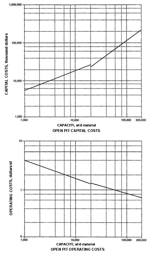
Two open pit models were developed, a small tonnage and a large tonnage model. The small tonnage model is valid for operations with daily capacities of 500 to 20,000 st/d of material moved (ore and waste). For the large tonnage model, applicable capacities are 20,000 to 200,000 st/d. A total of 11 mine capacities were used to develop cost estimates for the two models. Typically, small tonnage mines operate 1 or 2 shifts per day, 260 d/yr (5 d/wk), and large tonnage mines operate 3 shifts per day, 350 d/yr (7 d/wk). The models are based on the idealized shape shown in figure 1 (appendix B provides more detail). The pit bottom corresponds with the lower limit of the ore body to be mined.
Most recent open pit mining development in the United States has been for gold mining. The models are based on these types of mines and assume mine equipment used will be front-end loaders, hydraulic excavators, and diesel haul trucks. For large-scale mines in other commodities, such as copper, electric shovels tend to be used for excavation instead of front-end loaders or hydraulic excavators. Equipment used for the open pit models is shown in table 5. Equipment sizes, amounts, and cycle times were based on actual operations and equipment performance handbooks (15 - 17).
Figure 1. Open pit mine geometry.
Open pit mine geometry.
Front-end loaders are used for all loading at smaller mines, ranging in size from 4.5 cu yd (1,000 st/d) to 13.5 cu yd (20,000 st/d). Hydraulic excavators are used in conjunction with front-end loaders at many operations, and tend to be used exclusively for larger operations.
|
Table 5.-Typical equipment list, |
|
open pit models |
|
Equipment |
Size range |
|
Hydraulic excavators |
4.5 to 25 cu yd |
|
Front-end loaders |
4.5 to 13.5 cu yd |
|
Haul trucks |
35 to 150 st |
|
Bulldozers, D7-D11 |
200 to 770 hp |
|
Blasthole drills |
4-1/2 to 7-7/B in |
|
Graders |
135 to 275 hp |
|
Water trucks |
10,000 gal |
|
Explosive truck |
NAp |
|
Fuel-tube truck |
NAp |
|
Maintenance truck |
NAp |
|
Utility truck |
NAp |
|
Lights..... |
NAp |
|
NAp Not applicable. |
|
Sizes range from 4.5 cu yd (10,000 st/d) to 25 cu yd (100,000 st/d). Haul trucks vary in size from 35 to 150 st. Bulldozer sizes vary from 200 hp (D7) to 770 hp (D11).
Blasthole drills vary from 4-1/2 in to 7-7/8 in. A drill pattern of 13 by 16 ft was assumed, with a 20-ft bench height, a drill hole depth of 24 ft, and a powder factor of 0.45 lb ANFO per short ton. A quartzite host rock was assumed with a density of 2.225 st/bank cubic yard (BCY). Using a swell factor of 0.61, this yields 1.357 st/loose cubic yard (LCY). BCY is material in place (before blasting), LCY is broken or blasted material which contains more voids.
Capital and operating costs were estimated based on the assumptions listed above, and are summarized in tables 6 and 7. There are eight individual cost categories for both capital and operating costs, plus a total cost equation for each. Electrical costs are a small cost component for the open pit mine models and are included in the construction material category. Note that capital costs are expressed in dollars and operating costs in dollars per short ton of material (ore and waste) mined. All costs are based on daily capacity of the mine (X) in short tons per day of material (ore and waste) moved. Figure 2 summarizes the cost curves for the base case total cost equations.
|
Table 6. Small
open pit mine model, base case |
|
Category |
Capital cost, $ |
Operating cost, $/st |
|
Labor |
30,100(X)0.443 |
213(X)-0.610 |
|
Equipment |
121,000(X)0.516 |
0.513(X)-0.072 |
|
Steel |
2,930(X)0.525 |
0.110(X)-0.149 |
|
Fuel |
262(X)0.721 |
0.704(X)-0.159 |
|
Lube |
50.6(X)0.762 |
0.144(X)-0.110 |
|
Explosives |
24.0(X)0.963 |
0.221(X)-0.040 |
|
Tires |
16.5(X)0.904 |
0.509(X)-0.251 |
|
Construction material |
8,210(X)0.470 |
0.049(X)-0.037 |
|
Sales tax |
7,630(X)0.520 |
0.069(X)-0.084 |
|
Total |
160,000(X)0.515 |
71.0(X)-0.414 |
|
Table 7. Large
open pit mine model, base case |
|
Category |
Capital cost, $ |
Operating cost, $/st |
|
Labor |
405(X)0.443 |
21.5(X)-0.379 |
|
Equipment |
2,070(X)0.913 |
0.84(X)-0.128 |
|
Steel |
36.7(X)0.955 |
0.022(X)0.0 |
|
Fuel |
22.3(X)0.978 |
0.406(X)-0.103 |
|
Lube |
10.1(X)0.936 |
0.084(X)-0.065 |
|
Explosives |
30.2(X)0.941 |
0.147(X)0.0 |
|
Tires |
0.590(X)1.228 |
0.00015(X)0.546 |
|
Construction material |
51.8(X)0.965 |
0.034(X)0.0 |
|
Sales tax |
128(X)0.919 |
0.028(X)0.0 |
|
Total |
2,670(X)0.917 |
5.14(X)-0.148 |
|
X = Capacity of mine in short tons of ore and waste per day |
Appendix C provides an example problem applying the open pit cost equations for a large open pit mine from table 9. This example problem includes the use of haulage factors, which are discussed below.
HAULAGE ADJUSTMENT FACTOR
Haulage distance is one of the main variables in an open pit mine that will affect costs. Adjustment factors were developed for variations in haulage distance from the base cases. The geometry of the open pit was assumed to be an inverted frustum of a right circular cone (fig. 1), with the bottom of the pit at the lowest point of the ore body to be recovered. Surface topography is assumed to be level. Overall pit slope is 45°, and the in-pit haul road has an 8% (4.574°) grade. Haul distances were calculated from the centroid of the pit, based on a stripping ratio (SR) of 1:1, and the following assumptions for ore and waste haul distances:
waste haul = (depth to centroid/sin 4.574°) + (0.75r). (7)
ore haul = (waste haul distance) + 2,500 ft. (8)
Appendix B provides more detail on the mathematical relationships used for the open pit model.
Ore haul distances were varied to determine the relationship of haul distances to overall costs. Using equations 7 and 8 as a base case, the relationship of increased haul distances to costs were developed. These variations in cost are reflected in the haulage factors in tables 8 and 9. The first step in applying the haulage factors is to determine the average haul distance used for the base-case cost model. This average haul distance is found using equation 9 or 10 below, based on the assumptions in equations 7 and 8 (remember X = st/d material mined):
small open pit: av. haul distance, ore and waste (in ft)
(9)
large open pit: av. haul distance, ore and waste (in ft)
(10)
The haul factors are based on the average haul distance in excess of the base case, and are defined as d. If the average haul distance is less than the distance for the base case, use the base-case cost equations without adjustment (tables 6 and 7). For evaluations where the average haul distance is greater than the base case (equation 9 or 10), apply the haul factors in tables 8 and 9. A simple example will illustrate the procedure.
Figure 2.-Open pit capital and operating costs (average 1989 dollars).
-
|
Table 8. Small
open pit with haulage factors |
|
(Capacity range 1,000 - 20,000 st/d) |
|
Category |
Base case capital cost + haulage factor, $ |
|
Labor |
30,100(X)0.443 + 13,700(f/1000) |
|
Equipment |
121,000(X)0.516 + 344,000(f/1000) |
|
Steel |
2,930(X)0.525 + 1,400(f/1000) |
|
Fuel |
262(X)0.721 + 9,000(f/1000) |
|
Lube |
50.6(X)0.762 + 2,600(f/1000) |
|
Explosives |
24.0(X)0.963 |
|
Tires |
16.5(X)0.904 + 1,200(f/1000) |
|
Construction material |
8,210(X)0.470 + 25,200(f/1000) |
|
Sales tax |
7,630(X)0.520 + 22,300(f/1000) |
|
Total |
160,000(X)0.515 + 419,400(f/1000) |
|
|
|
|
Category |
Base case operating cost + haulage factor, $/st |
|
Labor |
213(X)-0.610 + 0.009(f/1000) |
|
Equipment |
0.513(X)-0.072 + 0.003(f/1000) |
|
Steel |
0.110(X)-0.149 |
|
Fuel |
0.704(X)-0.159 + 0.003(f/1000) |
|
Lube |
0.144(X)-0.110 + 0.001(f/1000) |
|
Explosives |
0.221(X)-0.040 |
|
Tires |
0.509(X)-0.251 + 0.003(f/1000) |
|
Construction material |
0.049(X)-0.037 |
|
Sales tax |
0.069(X)-0.084 |
|
Total |
71.0(X)-0.414 + 0.020(f/1000) |
|
f = Average
haulage distance in excess of base case, in feet (see equation 9) |
|
NAp = Not Applicable |
|
X = Capacity of mine in short tons of ore and waste per day |
|
Table 9. Large
open pit with haulage factors |
|
(Capacity range 20,000 - 200,000 st/d) |
|
Category |
Base case capital cost + haulage factor, $ |
|
Labor |
405(X)0.890 43,400+ (f/1000) |
|
Equipment |
2,070(X)0.913 + 527,000(f/1000) |
|
Steel |
36.7(X)0.955 + 2,100(f/1000) |
|
Fuel |
22.3(X)0.978 + 25,300(f/1000) |
|
Lube |
10.1(X)0.936 + 7,300(f/1000) |
|
Explosives |
30.2(X)0.941 |
|
Tires |
0.590(X)1.228 + 10,000(f/1000) |
|
Construction material |
51.8(X)0.965 + 53,900(f/1000) |
|
Sales tax |
128(X)0.919 + 35,600(f/1000) |
|
Total |
2,670(X)0.917 + 704,600(f/1000) |
|
|
|
|
Category |
Base case operating cost + haulage factor, $/st |
|
Labor |
21.5(X)-0.379 + 0.011(f/1000) |
|
Equipment |
0.840(X)-0.128 + 0.004(f/1000) |
|
Steel |
0.022(X)0.0 |
|
Fuel |
0.406(X)-0.103 + 0.004(f/1000) |
|
Lube |
0.084(X)-0.065 + 0.001(f/1000) |
|
Explosives |
0.147(X)0.0 |
|
Tires |
0.00015(X)-0.546 + 0.004(f/1000) |
|
Construction material |
0.034(X)0.0 |
|
Sales tax |
0.028(X)0.0 |
|
Total |
5.14(X)-0.148 + 0.024(f/1000) |
|
f = Average haulage distance in excess of base case, in feet (see equation
9) |
|
NAp = Not Applicable |
|
X = Capacity of mine in short tons of ore and waste per day |
Assume a deposit is being evaluated which will have an average haul distance (ore and waste) of 9,000 ft, and the operation will have a capacity of 50,000 st/d. As the capacity exceeds 20,000 st/d, use the large open pit model. Next, use equation 10 to determine the base case average = $55,862,405. haul distance = 145(50,000)°" = 6,901 ft. To find d, sub-tract the average haul distance for the deposit being evaluated from the average haul used for the base case: d = 9,000 - 6,901 = 2,099. Finally, using the variables X and d to determine the costs (for simplicity, only use the total cost equation in table 9):
Total capital cost
(11)
= $55,862,405
Total operating cost
(12)

= $1.09/st.
UNDERGROUND MINE MODELS
Each underground mining model includes the cost of development, daily production, and mine plant construction and operation. Using equation 4 or 5, daily mine capacity of ore can be calculated for an underground evaluation. Production from underground mines is usually mostly ore, so an evaluator can add,10% to the amount of ore mined (based on equation 4 or 5) to estimate the amount of waste. Most waste production is from drift and raise development. The equations are based on total production from the mine, assuming most of the material hauled (90%) is ore. Underground designs were based on case studies, WFOC files, and current rules-of-thumb for underground design (18-21).
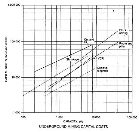
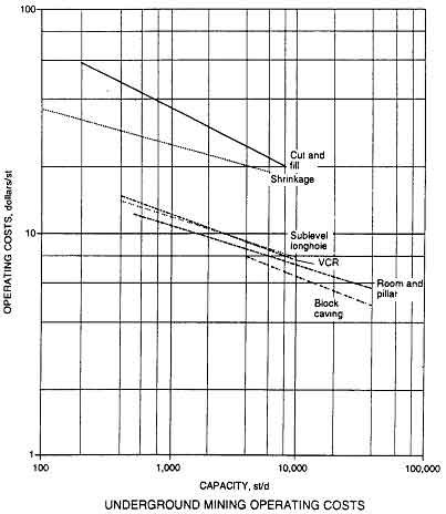
Figure 3 provides a series of cost curves summarizing the total cost equations for all underground models. Table 1 summarizes dilution and recovery factors common for each mining method included in this study. In addition, appendix D provides an example problem to demonstrate the use of the cost equations to estimate capital and operating costs of an underground mine, including the application of depth factors described below. Figures 4-9 are underground schematics for each of the underground methods, and are taken from previous Bureau publications (19, 22).
Figure 3.-Underground mining capital and operating costs (average 1989 dollars).
DEPTH FACTOR
Each underground mine model is based on an adit entry. For mines with shaft entry, the depth factors in table 10 must be added to the base cost curves (tables 1116). While some variability in costs would occur depending on depth of adits-inclines, the greatest variability occurs with shaft access. The depth factors are based on installing a production shaft, plus a combination ventilation shaft escapeway. For larger operations, the depth factor reflects the cost of additional shafts as needed. For depths greater than 500 ft, assume shaft entry to the ore body. Shaft access is often used for less than 500 ft depth also. The depth variable, D, is based on depth to bottom of ore body.
BLOCK CAVING MINE MODEL
Block caving requires a large capital expenditure for development and is usually applicable for large-scale projects. This method usually has a lower operating cost per short ton than any other underground method, and often the highest capital cost.
The ore body must have enough horizontal area to cave freely, without dilution from the sidewalls. Large massive deposits are most suited for block caving. Vein deposits must be wide-typically greater than 100 ft-with a steep dip. Ore grades should be fairly uniform, because this method does not allow much selectivity.
For this model, stope dimensions of 200 ft long by 70 ft wide by 300 ft high were assumed. Development of a typical stope includes a haulage drift, ventilation drift, Blusher drift, crosscuts-subdrifts, finger raises, access raises, and ore passes. Equipment requirements include jacklegs, fan drills, rockbolters, drift jumbos, Blushers, load-haul-dumps (LHDs), locomotives and rail cars, and miscellaneous support vehicles.
The model is valid for operations with daily mining capacities of 4,000 to 40,000 st/d. Base-case cost model equations are in table 11 and assume adit entry. For mines with shaft entry, apply the depth factors found in table 10.
|
Table 10. Underground
mine model depth factors |
|
(Capacity range 100 - 40,000 st/d) |
|
Category |
Capital cost, $ |
Operating cost, $/st |
|
Labor |
+ 75(D)(X)0.399 |
+ 2,010/(X) |
|
Equipment |
+ 350(X) + 65(D)(X)0.386 |
+ ).325(D)/(X) |
|
Steel |
+ 25(D)(X)0.373 |
+ 0.00014(D) |
|
Lumber |
NAp |
NAp |
|
Fuel |
NAp |
NAp |
|
Lube |
+ 6(D)(X)0.342 |
+ 0.090(D)/(X) |
|
Explosives |
+ 5(D)(X)0.389 |
NAp |
|
Tires |
NAp |
NAp |
|
Construction material |
+ 9(D)(X)0.522 |
+ 200/(X) |
|
Electricity |
+ 4(D)(X)0.230 |
+ 0.0014(D) |
|
Sales tax |
+ 21(X) + 6(D)(X)0.411 |
+ 133(X) + 0.025(D)/(X) + 0.00009(D) |
|
Total |
+ 371(X) + 180(D)(X)0.404 |
|
|
D = Depth of shaft to bottom of ore body in feet |
|
NAp = Not Applicable |
|
X = Capacity of mine in short tons per day |
|
Table 11. Block caving mine model, base case |
|
(Capacity range 4,000 - 40,000 st/d) |
|
Category |
Capital cost, $ |
Operating cost, $/st |
|
Labor |
27,900(X)0.646 |
60.0(X)-0.305 |
|
Equipment |
25,600(X)0.812 |
4.40(X)-0.230 |
|
Steel |
4,410(X)0.685 |
0.217(X)0.0 |
|
Lumber |
149(X)0.902 |
0.310(X)0.0 |
|
Fuel |
10.6(X)0.897 |
0.894(X)-0.239 |
|
Lube |
4.54(X)0.897 |
0.545(X)-0.253 |
|
Explosives |
1,040(X)0.737 |
0.183(X)-0.0 |
|
Tires |
1.87(X)0.946 |
0.412(X)-0.151 |
|
Construction material |
31,100(X)0.591 |
2.83(X)-0.182 |
|
Electricity |
50.4(X)0.748 |
1.36(X)-0.060 |
|
Sales tax |
2,590(X)0.779 |
0.350(X)-0.123 |
|
Total |
64,800(X)0.759 |
48.4(X)-0.217 |
|
X = Capacity of mine in short tons per day |
Figure 4. Block caving schematic. (Source: reference 19.)
-
-
CUT-AND-FILL MINE MODEL
The ore body is assumed to be vertical for application of the cut-and-fill mining model. Jackleg drills and stopers are used for production, with small jumbos used for drift development. Slushers move ore from the slope to ore chutes, LHDs move ore from chutes to ore storage pockets. Hydraulic sandfill is used to fill slopes.
This method is used where more selectivity is required than is possible with sublevel stoping or shrinkage stoping. This method provides good ore recovery and is adaptable to varying rock conditions. It is often used in deposits with weak wall rock, since the fill acts to support slope walls, in addition to providing a working platform for subsequent cuts.
The model is valid for operations with daily mining capacities of 200 to 8,000 st/d. Base-case cost model equations are in table 12, assuming adit entry. For mines with shaft entry, apply the depth factors found in table 10.
|
Table 12. Cut-and-fill
mine model, base case |
|
(Capacity range 200 - 8,000 st/d) |
|
Category |
Capital cost, $ |
Operating cost, $/st |
|
Labor |
16,700(X)0.673 |
158(X)-0.295 |
|
Equipment |
1,317,000(X)0.423 |
44.7(X)-0.499 |
|
Steel |
2,680(X)0.781 |
57.8(X)-0.474 |
|
Lumber |
652(X)0.532 |
2.81(X)-0.037 |
|
Fuel |
145(X)0.792 |
20.3(X)-0.604 |
|
Lube |
26.1(X)0.779 |
9.33(X)-0.539 |
|
Explosives |
2,220(X)0.793 |
4.72(X)-0.136 |
|
Tires |
247(X)0.834 |
1.16(X)-0.269 |
|
Construction material |
18,400(X)0.561 |
9.87(X)-0.151 |
|
Electricity |
25.3(X)0.843 |
94.6(X)-0.483 |
|
Sales tax |
73,400(X)0.446 |
3.38(X)-0.230 |
|
Total |
1,250,000(X)0.461 |
279(X)-0.294 |
|
X = Capacity of mine in short tons per day |
Figure 5. Cut-and-fill schematic. (Source: reference 22.)
ROOM-AND-PILLAR MINE MODEL
Room-and-pillar mining is usually applied where ore bodies are horizontal or have a flat dip (less than 30°). The model assumes use of jumbo drills for production and drift development. Rock bolts, in addition to pillars, are used for support of openings. Ore is moved by front-end
loaders, scoop trams, and trucks. Ore recovery is assumed to be 85% for an operation that planned to recover pillars later in the mine life. This method has a lower ore recovery than most underground methods and has very little dilution.
The model is valid for operations with daily mining capacities of 500 to 40,000 st/d. Base-case cost model equations are in table 13, assuming adit entry. For mines with shaft entry, apply the depth factors found in table 10.
|
Table 13. Room-and-pillar
mine model, base case |
|
(Capacity range 500 - 40,000 st/d) |
|
Category |
Capital cost, $ |
Operating cost, $/st |
|
Labor |
13,800(X)0.604 |
25.9(X)-0.216 |
|
Equipment |
55,800(X)0.664 |
1.49(X)-0.117 |
|
Steel |
9,350(X)0.559 |
1.94(X)-0.099 |
|
Lumber |
55.2(X)0.669 |
NAp |
|
Fuel |
1,280(X)0.561 |
0.984(X)-0.108 |
|
Lube |
354(X)0.561 |
0.541(X)-0.173 |
|
Explosives |
12,200(X)0.565 |
4.03(X)-0.100 |
|
Tires |
748(X)0.560 |
0.131(X)-0.080 |
|
Construction material |
4,120(X)0.653 |
0.024(X)-0.065 |
|
Electricity |
110(X)0.594 |
13.0(X)-0.490 |
|
Sales tax |
4,700(X)0.649 |
0.456(X)-0.102 |
|
Total |
97,600(X)0.644 |
35.5(X)-0.171 |
|
X = Capacity of mine in short tons per day |
Figure 6. Room-and-pillar schematic. (Source: reference 19.)
SHRINKAGE STOPE MINE MODEL
The shrinkage stoping model assumes a vertical ore body with moderate to strong ore and moderate to weak wallrock. Jackleg drills and stopers are used for production and drift development and rock bolts for wall support. LHDs move the ore. Recovery is assumed to be 90%, with 10% dilution. This method has a high recovery, but requires steep veins with a regular dip. Only enough ore is removed after each blast to provide a working platform for the next drill round; the remaining ore in the stope helps to support the wall rock. The remaining ore is removed from the slope at the end of the mining cycle, when support is no longer necessary.
This method is not as popular as it once was. Sublevel stoping, vertical crater retreat (VCR), sublevel caving, and cut-and-fill are all methods that can be applied to ore bodies where shrinkage stoping is feasible.
The model is valid.for operations with daily mining capacities of 100 to 6,000 st/d. Base-case cost model equations are in table 14, assuming adit entry. For mines with shaft entry, apply the depth factors found in table 10.
Figure 7. Shrinkage slope schematic. (Source: reference 19.)
|
Table 14. Shrinkage stope mine model, base case |
|
(Capacity range 100 - 6,000 st/d) |
|
Category |
Capital cost, $ |
Operating cost, $/st |
|
Labor |
34,100(X)0.643 |
41.0(X)-0.166 |
|
Equipment |
108,000(X)0.604 |
3.94(X)-0.263 |
|
Steel |
564(X)0.791 |
4.49(X)-0.073 |
|
Lumber |
249(X)0.858 |
3.73(X)-0.124 |
|
Fuel |
45.1(X)0.739 |
2.53(X)-0.379 |
|
Lube |
7.39(X)0.738 |
3.02(X)-0.460 |
|
Explosives |
1,200(X)0.765 |
4.94(X)-0.131 |
|
Tires |
63.3(X)0.771 |
0.933(X)-0.235 |
|
Construction material |
30,600(X)0.604 |
12.7(X)-0.289 |
|
Electricity |
38.2(X)0.854 |
3.82(X)-0.091 |
|
Sales tax |
8,220(X)0.613 |
1.57(X)-0.156 |
|
Total |
179,000(X)0.620 |
74.9(X)-0.160 |
|
X = Capacity of mine in short tons per day |
SUBLEVEL LONGHOLE MINE MODEL
The sublevel longhole mining method is used where the ore body is vertical or steeply dipping. Jumbo and down-the-hole drills are used for production, with small jumbos used for drift development. LHDs move the ore. Sublevels can be up to 150 ft apart. Development includes a haulage drift, raises for access to sublevels, sublevels for access to ore body, undercut below the stope, drawpoints, and a slot raise at the end of the stope.
The ore body must be vertical or steeply dipping. Both the hanging wall and footwall must be strong, since there is no support in the slopes. The ore must be competent, with regular boundaries.
The model is valid for operations with daily mining capacities of 400 to 10,000 st/d. Base-case cost model equations are in table 15, assuming adit entry. For mines with shaft entry, apply the depth factors found in table 10.
|
Table 15. Sublevel
longhole mine model, base case |
|
(Capacity range 400 - 10,000 st/d) |
|
Category |
Capital cost, $ |
Operating cost, $/st |
|
Labor |
16,500(X)0.599 |
37.0(X)-0.234 |
|
Equipment |
45,000(X)0.582 |
1.39(X)-0.118 |
|
Steel |
24,800(X)0.397 |
1.01(X)-0.007 |
|
Lumber |
6,240(X)0.357 |
0.184(X)0.0 |
|
Fuel |
453(X)0.580 |
0.830(X)-0.192 |
|
Lube |
194(X)0.580 |
0.360(X)-0.193 |
|
Explosives |
12,700(X)0.421 |
0.727(X)-0.010 |
|
Tires |
607(X)0.577 |
0.490(X)-0.107 |
|
Construction material |
19,400(X)0.509 |
3.73(X)-0.186 |
|
Electricity |
218(X)0.666 |
3.35(X)-0.325 |
|
Sales tax |
5,600(X)0.540 |
0.385(X)-0.079 |
|
Total |
115,000(X)0.552 |
41.9(X)-0.181 |
|
X = Capacity of mine in short tons per day |
Figure 8. Sublevel longhole schematic. (Source: reference 19.)
VERTICAL CRATER RETREAT MINE MODEL
The VCR mining method is used on vertical or steeply dipping ore bodies under similar conditions for sublevel stoping and shrinkage stoping. Down-the-hole drills are used for production, with small jumbos used for drift development. LHDs move the ore. Development includes a haulage drift, raises for access to drill overcuts, undercut of the complete area below the slope, drawpoints, and overcut of the complete slope area along the top of the slope. The VCR slopes are excavated in horizontal slices starting from the bottom, and the broken ore can remain in the slope for support similar to shrinkage stoping.
Figure 9. Vertical crater retreat schematic.
|
Table 16. Vertical
crater retreat mine model, base case |
|
(Capacity range 400 - 9,000 st/d) |
|
Category |
Capital cost, $ |
Operating cost, $/st |
|
Labor |
12,300(X)0.732 |
55.0(X)-0.306 |
|
Equipment |
20,300(X)0.770 |
1.83(X)-0.204 |
|
Steel |
277(X)0.843 |
0.607(X)-0.033 |
|
Lumber |
49.2(X)0.898 |
0.175(X)-0.018 |
|
Fuel |
18.5(X)0.798 |
1.05(X)-0.222 |
|
Lube |
8.03(X)0.798 |
0.450(X)-0.219 |
|
Explosives |
606(X)0.848 |
2.29(X)-0.042 |
|
Tires |
33.2(X)0.787 |
0.531(X)-0.160 |
|
Construction material |
12,500(X)0.650 |
3.78(X)-0.183 |
|
Electricity |
14.9(X)0.873 |
1.75(X)-0.078 |
|
Sales tax |
1,860(X)0.752 |
0.476(X)-0.097 |
|
Total |
45,200(X)0.747 |
51.0(X)-0.206 |
|
X = Capacity of mine in short tons per day |
MILL MODELS
Each mill model includes a simplified flowsheet to illustrate the main process steps for each mill. Flowsheets from existing operations were used as the basis for the mill models, augmented by current literature and design handbooks (23-31). Tailings pond costs are summarized in the following section. Figure 10 provides a series of cost curves summarizing the total cost equations for each mill model.
TAILINGS POND
Tailings ponds are required for most milling facilities. For the mill cost models, the cost of a tailings pond is required for all models except heap leach and solvent extraction-electrowinning. The size of tailings ponds and their containment dams varies widirly from one operation to another. This variability is dependent to a great extent on topography. For this reason, it is usually advisable to determine the specific areal requirements for tailings ponds for each individual project as it is evaluated.
The ore body must be vertical or steeply dipping. As with shrinkage stoping, the wallrock can be weak to moderate and the ore should be moderate to strong. The ore must be competent, with regular boundaries.
The model is valid for operations with daily mining capacities of 400 to 9,000 st/d. Base-case cost model equations are in table 16, assuming adit entry. For mines with shaft entry, apply the depth factors found in table 10.
In instances where this is not feasible, the following rough guidelines may be followed: for a 5-yr mine life17 acres per 1,000 st/d mill capacity, for a 10-yr mine life32 acres per 1,000 st/d mill capacity, and for a 20-yr mine life-62 acres per 1,000 st/d capacity (adapted from 32). It should be emphasized that these are guidelines to be followed only in the absence of specific data. It is much more accurate to study the topography of the area, choose the pond site, calculate the total tonnage and volume to be contained, and calculate the area requirements and amount of impoundment dam required for the site.
To calculate the costs, the total area of the pond and the linear feet of dam to be constructed are required. As a guideline, 1 acre is 43,560 ftz, which is 208.7 ft per square side. The assumed cross sectional area of the dam for the cost table is 27 ft high, 2,150 ft2 per linear foot (fig. 11). The total cost is the cost of preparing the tailings pond site plus the cost of constructing the impoundment dam around it. The cost for tailings pond site preparation includes the cost of installing 2,000 ft of slurry
Figure 10. Milling capital end operating costs (average 1989 dollars).
pipe and reclaim water pipe, which are included as lump sums in the labor and steel categories. A separate additional cost is included for ponds requiring hypalon liners and fencing. These costs are summarized in table 17.
Figure 11. Tailings dam cross section.
|
Table 17. Tailings
pond capital costs |
|
Category |
Tails pond |
Dam |
Liners1 |
|
|
($ + $acre) |
($/linear ft) |
($/acre) |
|
Labor |
30,200 + 502(A) |
45(L) |
9,500(A) |
|
Equipment |
502(A) |
45(L) |
NAp |
|
Steel |
109,200 |
NAp |
NAp |
|
Fuel |
601(A) |
55(L) |
NAp |
|
Lube |
148(A) |
13(L) |
NAp |
|
Construction material |
NAp |
NAp |
24,800(A) |
|
Sales tax |
6,600 + 30(A) |
3(L) |
1,490(A) |
|
Total |
146,000 + 1,783(A) |
161(L) |
5(L) + 35,790(A) |
|
A = Area of tailings pond in acres |
|
L = length of impoundment dam to construct around tailings pond in feet |
|
NAp = Not Applicable |
|
1 Liners are only required
in certain states. |
AUTOCLAVE-CIL-ELECTROWINNING
MILL MODEL
This model is designed for evaluating gold deposits containing sulfide (refractory) ore. The autoclave-carbon in leach (CIL)-electrowinning process is most often used for processing refractory gold ores with little or no byproducts. Autoclaves treat the ore by pressure oxidation, where the ore is subjected to elevated temperatures and pressures in an oxygen-rich environment. CIL circuits are often used where the ore contains preg robbing characteristics, such as fine clays or naturally occurring carbon within the ore. This method is also being used where short leach times are feasible. If a longer leach time is required, and no preg robbing characteristics are present in the ore, CIP would probably be applied. The cost equations are valid for ore tonnage capacities of 500 to 10,000 st/d. For this model, a grade of 0.09 oz/st Au was assumed, with a recovery of 90% Au. The CIL and autoclave-CIL models were developed from individual cost estimates prepared by Scott Stebbins.
Mine-run ore is initially crushed with a jaw, then a cone crusher. Crushed ore is then ground is a semiautogeneous grinding (SAG) mill and sent through cyclones. The oversize is sent to a ball mill, while the undersize is sent to a thickener. From the thickener the ore is sent to the autoclave circuit.
The thickened slurry is sent to a surge tank, then through a series of splash heating towers. It is then sent to the autoclaves. From the autoclaves, the slurry goes to flash cooling towers, a surge tank, cooling vessels, and on to the CIL circuit.
Carbon is added in the CIL circuit, which consists of a series of tanks with high efficiency agitators. Carbon is moved countercurrent to the slurry, which moves by gravity from the first to the last tank. Barren slurry from the last tank of the CIL circuit are sent to the tailings pond. The loaded carbon from the CIL circuit is sent to the stripping tanks. Pregnant strip solution is sent to the electrowinning circuit, where the electrowinning cells are used to plate gold onto steel wool cathodes. Loaded cathodes are removed, treated with dilute sulfuric acid, and sent to the refining furnace, where a dory is produced for shipment. Stripped carbon is regenerated in a kiln and returned to the circuit.
Figure 12 illustrates a simplified flowsheet for an autoclave-CIL mill flowsheet. Costs are summarized in table 18.
Figure 12. Autoclave-CIL-electrowinnlag mill flowsheet
|
Table 18. Autoclave-CIL-Electrowinning
mill model |
|
(capacity range 500 - 10,000 st/d) |
|
Category |
Capital cost, $ |
Operating cost, $/st |
|
Labor |
24,000(X)0.757 |
170(X)-0.433 |
|
Equipment |
40,300(X)0.780 |
4.42(X)-0.232 |
|
Steel |
16,300(X)0.773 |
0.147(X)0.0 |
|
Fuel |
NAp |
4.81(X)-0.087 |
|
Lube |
NAp |
5.00(X)-0.251 |
|
Construction material |
12,100(X)0.752 |
NAp |
|
Electricity |
NAp |
1.87(X)-0.059 |
|
Reagents |
NAp |
5.35(X)0.0 |
|
Sales tax |
4,110(X)0.774 |
0.467(X)-0.028 |
|
Total |
96,500(X)0.770 |
78.1(X)-0.196 |
|
NAp = Not Applicable |
|
X = Capacity of mill in short tons per day mill feed. |
CIL - ELECTROWINNING MILL MODEL
This model is designed for evaluating oxide gold deposits. The CIL-electrovvinning process is most often used for processing oxide gold ores with little or no byproducts. CIL circuits are often used where the ore contains preg robbing characteristics, such as fine clays or naturally occurring carbon within the ore. This method is also being used where short leach times are feasible. If a longer leach time is required, and no preg robbing characteristics are present in the ore, carbon-in-pulp (CIP) would probably be applied. The cost equations are valid for ore tonnage capacities of 500 to 10,000 st/d. For this model, a grade of 0.09 oz/st Au was assumed, with a recovery of 90% Au. The CIL and autoclave-CIL models were developed from individual cost estimates prepared by Scott Stebbins.
Mine-run ore is initially crushed with a jaw and cone crusher circuit. Crushed ore is then ground in a semi-autogenous grinding (SAG) mill and sent through cyclones. The oversize is sent to a ball mill, while the undersize is sent to the CIL circuit.
Carbon is added in the CIL circuit, which consists of a series of tanks with high efficiency agitators. Carbon is moved countercurrent to the slurry, which moves by gravity from the first to the last tank. Barren slurry from the last tank of the CIL circuit are sent to the tailings pond. The loaded carbon from the CIL circuit is sent to the stripping tanks. Pregnant strip solution is sent to the electrowinning circuit, where the electrowinning cells are used to plate gold onto steel wool cathodes. Loaded cathodes are removed, treated with dilute sulfuric acid, and sent to the refining furnace, where a dory is produced for shipment. Stripped carbon is regenerated in a kiln and returned to the circuit.
Figure 13 illustrates a simplified flowsheet for a CIL mill flowsheet. Costs are summarized in table 19.
Figure 13. CIL - electrowinning mill flowsheet
|
Table 19. CIL-electrowinning
mill model |
|
(Capacity range 500 - 10,000 st/d) |
|
Category |
Capital cost, $ |
Operating cost, $/st |
|
Labor |
15,800(X)0.715 |
451(X)-0.625 |
|
Equipment |
17,600(X)0.776 |
3.23(X)-0.236 |
|
Steel |
6,480(X)0.733 |
0.147(X)0.0 |
|
Lube |
NAp |
2.31(X)-0.343 |
|
Construction material |
9,380(X)0.709 |
NAp |
|
Electricity |
NAp |
2.07(X)-0.068 |
|
Reagents |
NAp |
3.44(X)0.0 |
|
Sales tax |
1,960(X)0.755 |
0.314(X)-0.031 |
|
Total |
50,000(X)0.745 |
84.2(X)-0.281 |
|
NAp = Not Applicable |
|
X = Capacity of mill in short tons per day mill feed. |
CIP - ELECTROWINNING MILL MODEL
This model is designed for evaluating oxide gold deposits. The CIP-electrowinning process is most often used for processing oxide gold ores with little or no byproducts. The cost equations are valid for ore tonnage capacities of 1,000 to 20,000 st/d. For this model, a grade of 0.1 oz/st Au was assumed, with a recovery of 89% Au.
Mine-run ore is initially crushed with a jaw, then a cone crusher. Crushed ore is then ground in a rod mill and sent through cyclones. The oversize is sent to a ball mill, while the undersize is sent to a thickener. The overflow from the thickener is sent to a series of carbon adsorption columns, while the underflow goes through a series of agitated leach tanks.
After leaching, the slurry is fed to the CIP circuit, which consists of a series of tanks with high efficiency agitators. Carbon is moved countercurrent to the slurry, which moves by gravity from the first to the last tank. Barren slurry from the last tank of the CIP circuit is sent to the tailings pond. The loaded carbon from the CIP circuit and the carbon columns is sent to the stripping tanks. Pregnant strip solution is sent to the electrowinning circuit, where the electrowinning cells are used to plate gold onto steel wool cathodes. Loaded cathodes are removed, treated with dilute sulfuric acid, and sent to the refining furnace, where a dote is produced for shipment. Stripped carbon is regenerated in a kiln and returned to the circuit.
Figure 14 illustrates a simplified flowsheet for a CIP mill flowsheet. Costs are summarized in table 20.
|
Table 20. CIP
mill model |
|
(Capacity range 1,000 - 20,000 st/d) |
|
Category |
Capital cost, $ |
Operating cost, $/st |
|
Labor |
114,800(X)0.527 |
484(X)-0.641 |
|
Equipment |
145,600(X)0.550 |
21.6(X)-0.463 |
|
Steel |
42,600(X)0.528 |
0.993(X)0.0 |
|
Lube |
NAp |
11.4(X)-0.463 |
|
Construction material |
55,800(X)0.543 |
NAp |
|
Electricity |
NAp |
26.8(X)-0.365 |
|
Reagents |
NAp |
2.75(X)0.0 |
|
Sales tax |
14,600(X)0.545 |
0.409(X)-0.057 |
|
Total |
372,000(X)0.540 |
105(X)-0.303 |
|
NAp = Not Applicable |
|
X = Capacity of ill in short tons per day mill feed. |
Figure 14. CIP mill flowsheet
COUNTERCURRENT DECANTATION-MERRILL
CROWE MILL MODEL
This model is designed for evaluating gold deposits. The vat leach-countercurrent decantation (CCD)-Merrill Crowe process is most often used for processing gold ores with high silver content relative to the gold. The cost equations are valid for ore tonnage capacities of 500 to 20,000 st/d. For this model, grades of 0.05 oz/st Au and 4.5 oz/st Ag were assumed, with recoveries of 93% Au and 75% Ag.
Mine-run ore is initially crushed with a jaw, then a cone crusher. Crushed ore is then ground in a ball mill and sent through cyclones. The oversize is returned to the ball mill, while the undersize is sent to a grinding thickener. The overflow from the thickener is also returned to the ball mill, while the underflow goes through a series of agitated leach tanks, where cyanide is added to the slurry.
After leaching, the slurry is fed to the CCD circuit, which consists of a series of thickener tanks. The pregnant solution overflows from the first tank to the pregnant solution tank. Barren solution is added to the last tank and flows countercurrent to the solids. The underflow solids from the last tank of the CCD circuit are sent to the tailings pond. The pregnant solution is pumped through clarifying filters and the solution sent to a clarified solution tank. The clarified solution is then deoxygenated in a vacuum tower and pumped to the precipitate filters. Barren solution from the filters is pumped to the last tank in the CCD circuit. The precipitate is sent to the refining furnace, where a dote is produced for shipment.
Figure 15 illustrates a simplified flowsheet for a CCD mill flowsheet. Costs are summarized in table 21.
|
Table 21. Countercurrent
decantation mill model |
|
(Capacity range 500 - 20,000 st/d) |
|
Category |
Capital cost, $ |
Operating cost, $/st |
|
Labor |
135,600(X)0.572 |
652(X)-0.664 |
|
Equipment |
155,300(X)0.588 |
22.8(X)-0.419 |
|
Steel |
42,000(X)0.619 |
0.894(X)0.0 |
|
Lube |
NAp |
12.0(X)-0.419 |
|
Construction material |
68,800(X)0.562 |
NAp |
|
Electricity |
NAp |
23.9(X)-0.308 |
|
Reagents |
NAp |
3.52(X)0.0 |
|
Sales tax |
15,800(X)0.589 |
0.541(X)-0.067 |
|
Total |
414,000(X)0.584 |
128(X)-0.300 |
|
NAp = Not Applicable |
|
X = Capacity of mill in short tons per day mill feed. |
Figure 15. Countercurrent decantation-Merrill Crowe mill flowsheet
FLOAT-ROAST-LEACH MILL MODEL
This model is designed for evaluating deposits where a gold ore requires fluid-bed roasting, typically carbonaceous or sulfide ore. The cost equations are valid for ore tonnage capacities of 1,000 to 20,000 st/d. For the model, a grade of 0.058 oz/st Au was assumed, with a recovery of 88%.
Mine-run ore is fed to a jaw crusher, then to a SAG mill for grinding. The ore is then run over a jig circuit to recover free gold. Tails from the jig are sent to a flotation circuit, which produces a concentrate and tailings. Tails from the flotation circuit are thickened and pumped to the tailings pond.
Sulfide concentrates from the flotation circuit are sent through cyclones, with oversize sent to a regrind mill. The
undersize from the cyclone, plus the material from the regrind mill, is thickened and dried in a disk filter. This dried sulfide concentrate is then delivered to the fluid-bed roaster. The resulting sulfide matte is then sent to a carbon column circuit, from which the loaded carbon is sent to stripping tanks. Pregnant strip solution is sent to the electrowinning circuit, where the electrowinning cells are used to plate gold onto steel wool cathodes. Loaded cathodes are removed, treated with dilute sulfuric acid, and sent to the refining furnace, where a dore is produced for shipment. Stripped carbon is regenerated in a kiln and returned to the circuit.
Figure 16 illustrates a simplified flowsheet for the float-roast-leach mill. Costs are summarized in table 22.
|
Table 22. Float-roast-leach
mill model |
|
(Capacity range 1,000 - 20,000 st/d) |
|
Category |
Capital cost, $ |
Operating cost, $/st |
|
Labor |
148,400(X)0.554 |
99.3(X)-0.370 |
|
Equipment |
178,000(X)0.560 |
115(X)-0.485 |
|
Steel |
62,100(X)0.530 |
NAp |
|
Fuel |
NAp |
0.620(X)0.0 |
|
Lube |
NAp |
70.0(X)-0.549 |
|
Construction material |
75,300(X)0.543 |
NAp |
|
Electricity |
NAp |
6.04(X)-0.223 |
|
Reagents |
NAp |
3.74(X)0.0 |
|
Sales tax |
18,800(X)0.551 |
1.30(X)-0.158 |
|
Total |
481,000(X)0.552 |
101(X)-0.246 |
|
NAp = Not Applicable |
|
X = Capacity of mill in short tons per day mill feed. |
Figure 16. Float-roast-leach mill flowsheet
FLOTATION MILL MODEL, ONE PRODUCT
This model is designed for evaluating deposits where a flotation mill will be used to produce one concentrate. The one-product flotation model is based on an operation producing a molybdenum concentrate. An evaluator should note that molybdenum mills have a higher reagent cost than most base metal flotation plants (i.e., copper, lead, or zinc). The model is valid for mill feed rates of 500 to 40,000 st/d. Typical recovery rates for base metal one-product flotation plants for copper, molybdenum, lead, or zinc are 90%.
Mine-run ore is initially crushed and sized in a series of crushers and vibrating screens to approximately minus 5/8 in. Crushed ore is then ground in rod mills and passed through cyclones. The oversize is ground in ball mills, then pumped back to the cyclones to achieve a minus 200 mesh flotation feed. Cyclone undersize is sent to the rougher flotation cells. These rougher concentrates pass to cleaner cells where they are further concentrated. Tails from the cleaner cells and middlings from the rougher cells are recirculated through the flotation circuit. Concentrates from the cleaner cells are thickened and dried prior to stockpiling for shipment. Tails from the rougher cells are sent to the tailings pond.
Figure 17 illustrates a simplified flowsheet for the one-product flotation mill. Costs are summarized in table 23.
|
Table 23. Flotation
mill model, one product |
|
(Capacity range 500 - 40,000 st/d) |
|
Category |
Capital cost, $ |
Operating cost, $/st |
|
Labor |
10,900(X)0.688 |
894(X)-0.708 |
|
Equipment |
26,700(X)0.684 |
21.0(X)-0.323 |
|
Steel |
9,470(X)0.622 |
0.742(X)0.0 |
|
Lube |
NAp |
2.07(X)-0.315 |
|
Construction Material |
42,200(X)0.653 |
NAp |
|
Electricity |
NAp |
1.55(X)-0.029 |
|
Reagents |
NAp |
0.771(X)0.0 |
|
Sales tax |
4,630(X)0.664 |
0.670(X)-0.158 |
|
Total |
92,600(X)0.667 |
121(X)-0.335 |
|
NAp = Not Applicable |
|
X = Capacity of mill in short tons per day mill feed. |
Figure 17. One-product flotation mill flowsheet
FLOTATION MILL MODEL, TWO PRODUCT
This model is designed for evaluating deposits where a flotation mill will be used to produce two concentrates. The two-product flotation model is based on an operation producing lead and zinc concentrates. The model is valid for mill feed rates of 500 to 40,000 st/d. Typical recovery rates for base metal two-product flotation plants for copper, lead, or zinc are 90%, 63% for molybdenum.
Mine-run ore is initially crushed and sized in a series of crushers and vibrating screens to approximately minus 5/8 in. Crushed ore is then ground in rod mills and passed through cyclones. The oversize is ground in ball mills, then pumped back to the cyclones to achieve a minus 200 mesh flotation feed. Cyclone undersize is sent to the first product rougher flotation cells. These rougher concentrates pass to cleaner cells where they are further concentrated. Tails from the cleaner cells and middlings from the rougher cells are recirculated through the first flotation circuit. Concentrates from the cleaner cells are thickened and dried prior to stockpiling for shipment.
Tails from the first product rougher cells flow to the second flotation circuit. Rougher concentrates are further treated in the second cleaner cells. As with the first product circuit, tails from the cleaner cells and middlings from the rougher cells are recirculated through the second product flotation circuit. Tails from the rougher cells are sent to the tailings pond, and the concentrates are thickened, dried, and stockpiled for shipment.
Figure 18 illustrates a simplified flowsheet for the two-product flotation mill. Costs are summarized in table 24.
|
Table 24. Flotation
mill model, two product |
|
(Capacity range 500 - 40,000 st/d) |
|
Category |
Capital cost, $ |
Operating cost, $/st |
|
Labor |
12,300(X)0.692 |
1,060(X)-0.719 |
|
Equipment |
30,400(X)0.691 |
25.2(X)-0.337 |
|
Steel |
8,170(X)0.658 |
0.742(X)0.0 |
|
Lube |
NAp |
2.63(X)-0.324 |
|
Construction material |
28,600(X)0.722 |
NAp |
|
Electricity |
NAp |
1.61(X)-0.027 |
|
Reagents |
NAp |
0.613(X)0.0 |
|
Sales tax |
3,970(X)0.704 |
0.796(X)-0.181 |
|
Total |
82,500(X)0.702 |
149(X)-0.356 |
|
NAp = Not Applicable |
|
X = Capacity of mill in short tons per day mill feed. |
Figure 18. Two-product flotation mill flowsheet
FLOTATION MILL MODEL, THREE PRODUCT
This model is designed for evaluating deposits where a flotation mill will be used to produce three concentrates. The three-product flotation model is based on an operation producing copper, lead, and zinc concentrates. The model is valid for mill feed rates of 500 to 40,000 st/d. Typical recovery rates for base metal three-product flotation plants for copper, lead, or zinc are 90%, 63% for molybdenum.
Mine-run ore is initially crushed and sized in a series of crushers and vibrating screens to approximately minus 5/8 in. Crushed ore is then ground in rod mills and passed through cyclones. The oversize is ground in ball mills, then pumped back to the cyclones to achieve a minus 200 mesh flotation feed. Cyclone undersize is sent to the first product rougher flotation cells. These rougher concentrates pass to cleaner cells where they are further concentrated. Tails from the cleaner cells and middlings from the rougher cells are recirculated through the first flotation circuit. Concentrates from the cleaner cells are thickened and dried prior to stockpiling for shipment.
Tails from the first product rougher cells flow to the second flotation circuit. Rougher concentrates are further treated in the second cleaner cells. As with the first product circuit, tails from the cleaner cells and middlings from the rougher cells are recirculated through the second
product flotation circuit. The concentrates from the cleaner cells are thickened, dried, and stockpiled for shipment.
Tails from the second product rougher cells flow to the third flotation circuit. Rougher concentrates are further treated in the third cleaner cells, while tails from the cleaner cells and middlings from the rougher cells are recirculated through the third product circuit. Third product concentrates from the cleaner cells are thickened, dried, and stockpiled. Tails from the rougher cells are sent to the tailings pond.
Figure 19 illustrates a simplified flowsheet for the three-product flotation mill. Costs are summarized in table 25.
|
Table 25. Flotation
mill model, three product |
|
(Capacity range 500 - 40,000) st/d) |
|
Category |
Capital cost, $ |
Operating cost, $/st |
|
Labor |
12,700(X)0.696 |
1,200(X)-0.725 |
|
Equipment |
31,600(X)0.694 |
29.6(X)-0.3348 |
|
Steel |
6,240(X)0.694 |
0.742(X)0.0 |
|
Lube |
NAp |
3.20(X)-0.330 |
|
Construction material |
29,800(X)0.725 |
NAp |
|
Electricity |
NAp |
1.66(X)-0.027 |
|
Reagents |
NAp |
1.13(X)0.0 |
|
Sales tax |
4,020(X)0.710 |
0.852(X)-0.165 |
|
Total |
83,600(X)0.708 |
153(X)-0.344 |
|
NAp = Not Applicable |
|
X = Capacity of mill in short tons per day mill feed. |
Figure 19. Three-product flotation mill flowsheet.
GRAVITY MILL MODEL
This model is designed for evaluating deposits where a gravity mill will be used to process ore that can be separated by gravity. Typical deposits where gravity mills are used include free milling gold, some tungsten, and other heavy mineral deposits. The model is valid for feed rates of 100 to 1,000 st/d. Recovery is assumed to be 93%.
Mine-run ore is initially crushed by a jaw crusher. The discharge is sent to a double-deck screen, where the plus 3/4 in fraction discharges onto a conveyor and is fed to a cone crusher. The minus 3/4 in fraction from the jaw and cone crusher is conveyed to vibrating screens. Oversize from the screens is returned to the cone crusher, and the undersize is slurried and fed to the jig.
Tails from the jig go to the rod mill, where grinding occurs in closed circuit with a cyclone classifier. Overflow from the cyclone is pumped to a spiral classifier. Size fractions from the classifier are sent to a series of tables to produce a high-grade concentrate, a middling product, and tailings. The middlings are combined and recycled through the rod mill.
Table concentrates are sent to a flotation cell where any sulfides present are floated off. Underflow from the float cell is combined with the concentrates from the jig and then thickened and dried. Tailings are thickened and sent to the tailings pond.
Figure 20 illustrates a simplified flowsheet for the gravity mill. Costs are summarized in table 26.
|
Table 26. Gravity
mill model |
|
(Capacity range 100 - 1,000) st/d) |
|
Category |
Capital cost, $ |
Operating cost, $/st |
|
Labor |
45,200(X)0.544 |
41.0(X)-0.383 |
|
Equipment |
57,500(X)0.509 |
18.6(X)-0.408 |
|
Steel |
17,500(X)0.515 |
1.22(X)-0.112 |
|
Lube |
NAp |
1.16(X)-0.423 |
|
Construction material |
10,700(X)0.574 |
NAp |
|
Electricity |
NAp |
9.32(X)-0.408 |
|
Reagents |
NAp |
0.208(X)0.0 |
|
Sales tax |
5,110(X)0.521 |
0.980(X)-0.316 |
|
Total |
135,300(X)0.529 |
67.8(X)-0.364 |
|
NAp = Not Applicable |
|
X = Capacity of mill in short tons per day mill feed. |
Figure 20.-Gravity mill flowsheet
HEAP LEACH MILL MODEL
This model is designed for evaluating deposits where a heap leach operation will be used to process gold and/or silver ore. Typical deposits where heap leaching is used are low-grade gold and silver oxide deposits. For this model, a gold deposit with a grade of 0.04 oz/st Au was assumed, with a recovery of 70%. The cost equations are valid for ore tonnage capacities of 1,000 to 20,000 st/d.
Mine-run ore is crushed in a jaw and cone crusher in series, screened, and stored in a fine ore bin. Trucks haul the ore to the heap leach pads, where bulldozers are occasionally used to contour or level the pile. A cyanide leach solution is sprayed on the leach pads, which percolates through the ore and is collected in a pregnant solution pond. Leached ore is washed and then moved to waste dumps. The pregnant solution is pumped to a series of carbon adsorption columns. Barren solution from the columns is returned to the leach pads. The loaded carbon is sent to stripping tanks. Pregnant strip solution from the tanks is sent to the electrowinning cells, where the gold is plated onto steel wool cathodes. Loaded cathodes are removed, treated with dilute sulfuric acid and sent to the refining furnace, where a dory is produced for shipment. Stripped carbon is regenerated in a kiln and returned to the circuit.
Figure 21 illustrates a simplified flowsheet for the heap leach mill. Costs are summarized in table 27.
|
Table 27. Heap leach mill model |
|
(Capacity range 1,000 - 20,000 st/d) |
|
Category |
Capital cost, $ |
Operating cost, $/st |
|
Labor |
316,200(X)0.583 |
135(X)-0.562 |
|
Equipment |
60,100(X)0.629 |
5.50(X)-0.357 |
|
Steel |
47,900(X)0.372 |
NAp |
|
Fuel |
NAp |
0.266(X)-0.013 |
|
Lube |
NAp |
2.91(X)-0.350 |
|
Tires |
NAp |
0.071(X)0.0 |
|
Construction material |
41,500(X)0.452 |
1.08(X)0.0 |
|
Electricity |
NAp |
13.7(X)-0.491 |
|
Reagents |
NAp |
1.30(X)0.0 |
|
Sales tax |
6,610(X)0.583 |
0.231(X)-0.040 |
|
Total |
296,500(X)0.512 |
31.5(X)-0.223 |
|
NAp = Not Applicable |
|
X = Capacity in short tons per day mill feed. |
Figure 21.-Heap leach mill flowsheet
SOLVENT EXTRACTION-ELECTROWINNING
MILL MODEL
This model is designed for evaluating deposits where a solvent extraction-electrowinning (SX-EW) mill will be used to produce a copper cathode product. Typical applications of SX-EW mills are for leach solutions from oxide or chalcocite dump, waste, or in situ copper ores. The cost equations are valid for ore tonnage capacities of 6,000 to 70,000 st/d. Basic assumptions include an ore grade of 0.4% Cu and a recovery of 50%. The cost equations are based on X in st/d to be consistent with other cost sections. SX plants are usually expressed in gallons per minute (gal/min), and EW plants in lb/d Cu produced. For this model, to convert to lb/d Cu: (X)(4.0) = lb/d Cu produced. To convert to gal/min: (X)/15 = gal/min feed to plant.
The model is based on a typical configuration of heap leach pads, two extraction stages, and one strip stage. Pregnant leach solution is pumped to the solvent extraction circuit from the solution ponds. In the first extraction stage, mixer-settler solution is mixed with organic flowing from the second stage, extracting some of the copper. The solution is pumped to the second extraction stage where it is mixed with freshly stripped organic to recover the remaining copper. The barren solution (raffinate) flows from the second stage to the leach dumps.
The loaded organic is sent from the extraction section to the stripping section, where it is mixed with an acidic electrolyte from the electrowinning circuit. This electrolyte strips the copper from the organic phase. After the mixture separates in settling tanks, the barren organic is returned to the second extraction stage. The coppercontaining electrolyte flows to the strong electrolyte tanks, from which it is pumped to electrolyte filters to remove entrained organic. The clarified strong electrolyte is then fed to the electrowinning circuit.
The strong electrolyte passes through electrolyte interchangers, where heat from outgoing spent electrolyte preheats the incoming strong electrolyte. The strong electrolyte then goes to a circulation tank, where it is mixed with spent electrolyte from the electrowinning cells. Feed electrolyte is pumped continuously from the tank to the electrolytic cells. Electrolysis occurs in the cells, where insoluble lead-based anodes are used, and the copper is plated on cathodes of stainless steel or thin copper starter sheets.
Figure 22 illustrates a simplified flowsheet for the SXEW plant. Costs are summarized in table 28. Since SX costs tend to vary in a typical geometric regression form, and the EW cost component of the plants tend to have a
linear relationship, the capital cost equations in table 28 are in the form of the SX component plus the EW component to calculate the total SX-EW capital cost. To convert the costs expressed in $/st to $/lb Cu produced: ($/st)/4.0 = $/lb Cu produced.
|
Table 28. Solvent-extraction-electowinning mill model |
|
(Capacity range 6,000 - 70,000 st/d) |
|
Category |
Capital cost, $ |
Operating cost, $/st |
|
Labor |
2,510(X)0.571 + 89(X) |
0.499(X)-0.146 |
|
Equipment |
4,810(X)0.600 + 228(X) |
0.248(X)-0.144 |
|
Steel |
1,030(X)0.590 + 44(X) |
0.105(X)-0.144 |
|
Lube |
NAp |
0.058(X)-0.151 |
|
Construction material |
5,640(X)0.602 + 272(X) |
NAp |
|
Electricity |
NAp |
1.45(X)-0.145 |
|
Reagents |
NAp |
0.583(X)-0.143 |
|
Sales tax |
688(X)0.600 + 32(X) |
0.056(X)-0.144 |
|
Total |
14,600(X)0.596 + 665(X) |
3.00(X)-0.145 |
|
NAp = Not Applicable |
|
X = Capacity of mill in short tons per day mill feed. |
|
NOTE: SX plant gal/min = (X)/15 |
|
EW plant lb Cu produced = (X)(4.0) |
Figure 22. Solvent extraction-electrowlnning mill flowsheet (Source: adapted from reference 29.)
SUMMARY
The use of these simplified cost models will allow an evaluator to make a quick prefeasibility type estimate for a mineral deposit. Capital and operating costs for a mine and mill can be estimated based on capacity of the operation in short tons per day. Adjustment factors are provided for haulage distance variation in open pits and
variability of depth to bottom of ore body for underground mines. Guidelines for calculating daily capacity based on reserve tonnage are provided. Additionally, guidelines for estimating the costs of tailings ponds, powerlines, and road construction are included.