
By Valerie J. Kelly, Richard P. Hooper, Brent T. Aulenbach, and Mary Janet
Sample Collection and Laboratory Analysis || Quality Assurance Program || Flux Calculation || Yield Calculation
Sample Collection and Laboratory Analysis
Standard USGS protocols, described by Edwards and Glysson (1988), were used for the collection of depth- and width-integrated samples at all stations. For most stations, samples were collected from a boat, but a few stations were sampled from cableways (in the upper Mississippi, Colorado, and Rio Grande Basins), from a bridge (Platte River), or by wading (lower Rio Grande). A minimum of two people collected the sample to minimize the opportunity for contamination of low-concentration analytes, following the protocols of Horowitz and others, 1994. Samples were processed according to established USGS protocols (USGS, 1997-99).
The USGS National Water Quality Laboratory in Denver, Colorado, analyzed all samples for the various dissolved and whole-water constituents using documented USGS methods and quality-assurance practices (Brenton and Arnett, 1993; Burkhardt and others, 1997; Faires, 1993; Fishman and Friedman, 1989; Fishman, 1993; Garbarino, 1999; Patton and Truitt, 2000; Struzeski and others, 1996; Zaugg and others, 1995). Method codes for each constituent analysis are provided in the water-quality data tables. An ASCII text file containing references for laboratory methods for each analyte, defined by method codes where appropriate, is provided. Routine suspended sediment concentrations were determined by using gravimetric methods (separation by filtration or evaporation, as appropriate) by as many as seven different USGS laboratories through WY97. In WY98, sediment analyses were centralized so that all samples from a given basin were sent to a single laboratory. Chemical analyses of suspended sediment, including sediment concentration, were performed after total digestion of the dewatered sediment (separation by flow-through centrifuge) at the USGS laboratory in Atlanta, Georgia. Methods are provided by Horowitz et al. (2001a). Horowitz and others (2001a) compares sediment concentration data obtained from the gravimetric versus the centrifuge separation.
The NASQAN Quality Assurance (QA) program was developed to support the data quality objective of annual flux estimation. NASQAN has a highly dispersed team of field personnel because of the national scale of the network. Therefore, ensuring consistency across the network is a critical element of the QA program. Major QA elements include well-defined protocols for sample collection, sample processing, chemical analysis, and data review. Extensive training is provided for field personnel to ensure that uniform procedures are used in sample collection and processing, and that data review is conducted according to established data-quality criteria. A field audit of all sampling crews was performed early in the program by each basin coordinator.
Quality-Control Data
An additional component of the QA program consists of the collection and evaluation of quality control (QC) samples, including blanks, replicates, and field-matrix spikes for pesticides. Data from these samples document the performance of the overall process of sample collection, processing, and analysis. Quality-control samples typically comprise 10-20 percent of the total number of samples submitted for analysis.
Blanks
Blank samples are prepared from production lots of deionized water that are certified to be free of the analytes of interest, and are used to document the potential for contamination from a variety of sources. While several kinds of blank samples were collected for the NASQAN program, only data for field blanks are included in this report. Field blanks are prepared and processed under the same routine field conditions used for stream samples. These samples are used to identify and quantify any contamination arising collectively from all sources related to sampling, processing, shipping, and analysis.
Field blank samples were collected at all NASQAN stations for all constituents, with the exception of suspended sediment and sediment chemistry. The frequency of blank sample collection varied with constituent group, ranging from about 20 percent of routine environmental or ambient samples for trace elements, to about 15 percent for nutrients, carbon, and major ions, and 10 percent for pesticides.
Analysis of results for blank samples was conducted by comparing the distribution of blank results to the ambient data for each station and parameter combination. Detectable concentrations in the blank samples were considered to be significant when they exceeded both twice the minimum reporting level and 10 percent of the mean ambient data.
Replicates
Replicate samples are collected and processed so that the two separate samples are essentially identical. In the NASQAN program, all routine replicate samples were collected as concurrent replicates; that is, two separate samples were collected and processed concurrently, rather than splitting a single sample. These samples provide a measure of the variability inherent in the entire process of sample collection, processing, and analysis. To measure the variability due to sample processing and analysis alone, a single set of split replicate samples was collected at every station during 1997. The split replicate samples were collected as a single volume of water that was subsequently split in the field into replicate samples.
Generally, two to three replicate samples were collected annually at every station for every constituent group. Because of concerns regarding variability in suspended sediment concentrations, sediment replicates were collected for nearly every sample beginning in 1998.
Analysis of results for replicate samples was conducted by comparing the variability of replicate samples to that for the routine samples. Ratios of standard deviations from both concurrent and split replicates relative to those from routine samples were evaluated to determine the relative importance of sampling variability to overall variability in the measurement process. Differences in results for each replicate pair were also evaluated by percent relative difference to indicate the reproducibility of analytical results for samples collected and processed in essentially identical manner.
Field-Matrix Spikes
Field spikes are samples fortified with known concentrations of a group of analytes. These samples are paired with unspiked samples in order to measure the potential bias due to matrix interference with the analytical method. Field spike samples were collected for pesticides only, generally once/year at every station. Concentrations in the routine spike mixture represented an increase of about 0.1 microgram per liter (ug/L) over that of the unspiked stream sample. Because ambient pesticide concentrations at some stations can exceed the routine spike level by one to two orders of magnitude, several sets of high-spike samples were also collected at a subset of stations to evaluate the potential for matrix interference at higher concentration ranges.
Percent recoveries for the spiked analytes were calculated as the ratio of the difference between the spiked and unspiked concentrations to the concentration of the added spike. Determination of recover efficiencies allows an evaluation of how well the analytical method can quantify material present at a know concentration in the ambient stream matrix. Recoveries less than or greater than about a 20 percent deviation from 100 percent recovery may indicate analytical interference from some constituent or group of constituents within the sample.
Data Quality
For the purpose of consistent data review, data quality criteria have been defined by the NASQAN program, and provide the basis for national data review procedures. The criteria are based on various ranges of statistical variation, including the distribution of previous data for the site, where available. NASQAN maintains a web-based interactive review process wherein questionable data are flagged for special review and input by District personnel. The data tables published in this report contain data-quality indicator (DQI) codes of "Q" for all constituents where exceedances occur for NASQAN criteria. Note that this DQI code is generated from the simple comparison of sample data to the statistical criteria, and does not necessarily imply that the data are questionable. In many cases, data are flagged simply because they represent extreme conditions, which are targeted by the NASQAN sampling strategy. A lookup table (RDB format) with data that exceed the NASQAN criteria, and input from the districts where available, is provided for additional context, especially information about laboratory verification of questionable values and hydrologic conditions during sample collection.
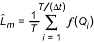
Fluxes for major ions, sediment, dissolved trace elements, and nutrients were estimated using the LOADEST2 computer program (Crawford, 1996). LOADEST2 is based on the rating-curve (regression) method (Crawford, 1991), and estimates the mean flux for a specified period according to the following generic equation, with units defined for annual flux calculation:
 (1)
(1)
where LM is the estimated mean flux (i.e. daily mean),
T is the time period (i.e. one year or 365 days),
Delta t is the fixed sampling interval, (i.e. one day)
Qi is streamflow (mean daily) at time i; and
f(Qi) is the flux estimated from the rating curve at time i (i.e. for a given day).
The generic rating curve equation f(Qi) has the form:
ln( L ) = a0 + a1 ln( Q ) + a2 ln( Q )2 + a3sin( t ) + a4cos( t ) + a5t (2)
where L is flux,
Q is streamflow,
t is time, and
a0...a5 are the estimated regression parameters.
For each station/water-quality-parameter combination, LOADEST2 determines which parameters in equation 2 to include in the rating curve. In all cases, the intercept term (a0) and the flow term, a1ln(Q), are included, and the seasonal terms, a3sin(t) and a4cos(t), are either included or excluded as a pair. Aikaike's information criterion is used as a measure to select the best-fit model (Judge et al., 1985). Aikaike's information criterion attempts to achieve the goal of explaining as much variance as possible while minimizing bias. This is accomplished by balancing the inclusion of more variables to minimize the variance of the estimates with the inclusion of fewer variables to simplify the data requirements (Helsel and Hirsch, 1992). Aikaike's information criterion is similar to Mallow's Cp (Neter and others, 1985) but is suitable for use with censored values (concentrations below the reporting or detection limit).
Constituent fluxes published in this report were generated using the linear-attribution (LA) method in LOADEST2. LA is based on a linear least-squares regression to minimize the sum of the squared differences between the observed and predicted values. The Duan method, which is a nonparametric method, is used for bias-correction when variables are transformed prior to the regression (Duan, 1983). Censored values are iteratively estimated until the sum of squares is minimized (Chatterjee and McLeish, 1986). LA is the preferred method because it uses the more common least-squares approach and a nonparametric transformation bias-correction. Furthermore, it does not require that the residuals be normally distributed.
Model parameters determined by LOADEST2 are provided for all stations and constituents, as appropriate. Limited model diagnostic information is also provided, including whether the data were sufficient to generate a model and whether convergence was obtained. In LOADEST2, for linear attribution, convergence is obtained when the sum of squares for the current iteration differs from the sum of squares for the previous iteration by less than a small fraction of the value of the current sum of squares (1/1E6) after 250 iterations. If convergence is not obtained, the model issues a warning; parameters are not presented in this report if the model does not converge. The most probable reason for a model to fail to converge is the lack of a single solution due to a very large percentage of censored data.
LOADEST2 was not used for estimating the flux of pesticides. The concentration/discharge relation, generally, is not stable for man-made, applied chemicals, but, instead, will vary depending upon the relation of storm runoff to application periods of these chemicals. For these cases, a period-weighted approach was used in which concentrations between sampling visits were linearly interpolated through time and multiplied by mean daily discharge. The emphasis on high-discharge sampling periods in the design of NASQAN may bias the fluxes calculated with this method. Censored values were handled by bounding the flux estimates: a minimum flux is defined by setting censored values to zero, and a maximum flux is defined by setting censored values to their reporting limit. In this report, the minimum period-weighted flux only is reported for pesticides.
Similarly, because the concentration of sediment-associated trace elements was not related to either the sediment concentration or to stream discharge, LOADEST2 was not directly used to determine their flux. Rather, the sediment flux (determined by LOADEST2) was multiplied by the median concentration of the constituent of interest to calculate the sediment-associated trace element flux. The flux estimates presented in this report differ somewhat from those contained in Horowitz and others (2001a) primarily because they are based on a different period of sediment record. Flux estimates are sensitive to a number of decisions, including the calibration strategy as well as the calibration methodology. For this report, sediment concentrations measured between water years 1996-2000 only were used to calibrate the sediment concentration model (equation 2), whereas Horowitz and others (2001a) used the entire historical record for calibration. This approach was taken for consistency because the report focuses on the period 1996-2000 for all other flux estimates.
Finally, LOADEST2 was not suitable for calculation of flux for suspended organic carbon (SOC). Because of limitations of the analytical method, many values for SOC were censored on the high end, that is, values were reported as greater than the upper limit of the calibration curve for the analysis. For this reason, fluxes for SOC are not included in this report.
Although fluxes were determined for every day, only annual fluxes are reported, as the standard errors of these values are much smaller than for the daily values. Typically, the standard error of annual fluxes are between 10 and 30 percent of the flux estimate, whereas the standard error of the daily values are often in excess of 100 percent. See Horowitz and others (2001b) for further discussion of the influence of temporal resolution on the uncertainty of flux estimates.
Yields, defined as flux per unit area, are useful for comparing relative contributions of constituents from different basins having variable geology, land use, and chemical application rates. To determine the incremental yield of a specific subbasin, the upstream fluxes are subtracted from the subbasin outlet flux, and this difference is divided by the basin area. Basin areas do not include non-contributing areas, as listed in USGS station files. LA was used for all yield determinations where possible. If the model did not converge, then the minimum period-weighted approach was used.
If stream discharge decreased downstream, these losses were assumed to result from diversion of water either out of the basin or to irrigation. Solutes were assumed to be transported proportionally with the diverted water, so that a loss of constituent mass from the river system was calculated. Therefore, total basin export was calculated as the sum of export from terminal station(s) and these losses. Both the Rio Grande and Mississippi have two terminal stations (Table I).
The incremental yield for the Red River Basin (Figure 1) requires a more complicated calculation because of the diversion of Mississippi River water to the Atchafalaya River through the Old River Control structure. The quantity of this diversion is measured; however, no water-quality samples were collected at this site. The concentration of dissolved constituents at the Old River Control structure was assumed to be equal to the concentration at Saint Francisville, about 50 km downstream. The Red River incremental flux is calculated as the difference between the flux measured at the Atchafalaya River and the inferred flux at the Old River Control structure. The flux for the lower Mississippi River is the sum of the flux measured at St. Francisville and the inferred flux at the Old River Control structure.
Continue to Results or Return to Table of Contents